External noise
External noise is the noise external to the receiver system.
(ITU-R 2015) gives some guidance on expected ambient noise.
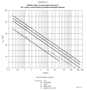
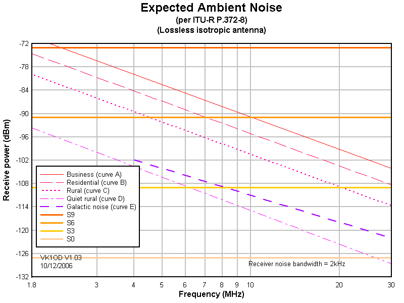
Above is Figure 10 which gives guidance on the expected median ambient noise figure.
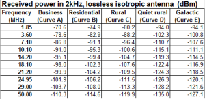
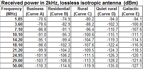
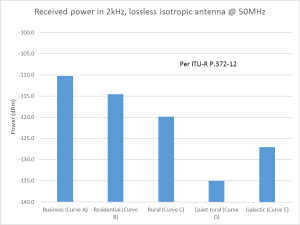
The table above gives calculates noise power in a 2kHz bandwidth receiver with lossless antenna system for the lower ham bands from the equations given in (ITU-R 2015). Note that the medians vary somewhat with location and time, see (ITU-R 2015).
From the table, business (city) man made noise (A) is 17dB higher than galactic (E), and rural (C) is 7dB higher than galactic. Unless there is some ionospheric absorption occurring, you are unlikely to observe noise below galactic level.
Noise can be expected to vary by hour of day, from day to day, and season to season. Importantly, noise may vary with direction, eg pointing through busy roads, office buildings, shopping centres etc, neighbouring buildings, powerlines etc.
Measurement of external noise is not too difficult, but rarely do hams understand quantitatively their own noise environment.
Internal noise
Noise contributed by the various stages of a receiver system can be reduced to an equivalent input noise at the input of a noiseless receiver, and that is often expressed in the form of the receiver Noise Figure.
A typical receiving system for 6m would have a noise figure around 6dB (at the antenna connector). As will be seen, there is little need for better noise figure.
The noise floor of a receiving system with NF=6dB (4.5dB receiver and 1.5dB line loss) is -135dBm. In such a receiver, AGC action is typically delayed until the signal is around 25dB above the noise floor, around -110dBm in this case. There will be no S meter deflection in traditional receivers below AGC onset.
Above, the median expected noise falls below the typical AGC threshold (S meter threshold) for the example receiver (-110dBm), and apart from Curve A, the noise may not cause S meter deflection.
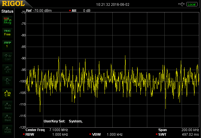
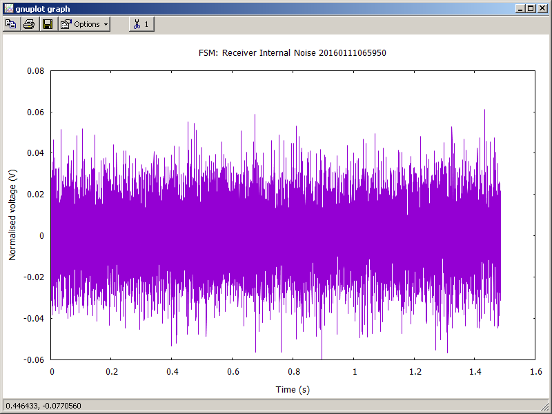
In a single isolated measurement at my location, I measured -123dBm which is in the range expected of a semi rural residential with underground power.
Receivers with an additional preamp may show significant S meter deflection, the preamp will increase gain without significantly improving S/N ratio, indeed they may degrade S/N ratio.
Total noise power
The internal and external noise power add, but it is the power in watts or in equivalent temperature that can be added, not the dBm figure.

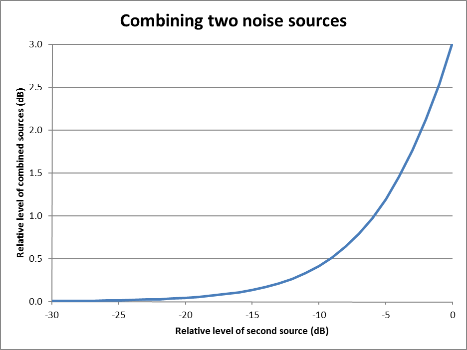
The chart above shows the effect of combining two additive power values. If they differ by more than 20dB, the sum is within 0.05dB of the higher power. For lesser ratios, the weaker power needs to be factored in, and the graph provides a simple means if you don’t want to crunch the numbers.
For example, if we took the median power in a quiet rural precinct from the table above to be -119.9dBm, and noise floor to be -135dBm, looking up -135–119.9=-15.1dB on the horizontal axis we see that the combined power is 0.15dB more than the higher power, so -119.1+0.15=-119.8dBm. This is unlikely to cause S meter deflection most of the time as the median is almost 10dB lower than AGC onset.
Working the numbers for residential precinct from the table above to be -114.6dBm, and noise floor to be -135dBm, looking up -135–114.6=-20.4dB on the horizontal axis we see that the combined power is 0.05dB more than the higher power, so -114.6+0.05=-119.8dBm., -114.6. This is likely to cause S meter deflection occasionally as the median is just 5dB lower than AGC onset.
Low noise antennas
One of the recent market directions is so-called low noise antennas. The term is used to describe directional antennas with reduced side lobe response inspired perhaps by (Bertelsmeier 1987) who contrived a rather naive statistic based on the noise power captured by a Yagi in free space tilted up 30° from the Z=0 plane and excited by two arbitrary noise scenarios in the upper and lower hemispheres, the statistic labelled G/Ta, transformed by others to G/T in ignorance of the true meaning of the industry term G/T.
Reduced side lobe response sounds a good idea, but what is the expected impact on total external noise power received?
For a Yagi in free space, if the distribution of external noise is uniform in three dimensional space:
- the same noise power will be received irrespective of the pointing of the antenna; and
- a lossless antenna captures the same amount of noise power irrespective of its gain.
But we are not in free space, are we.
For Yagi pointing horizontally over flat ground, if the distribution of external noise is evenly distributed over all azimuth headings:
- the same noise power will be received irrespective of the pointing of the antenna; and
- a lossless antenna captures the same amount of noise power irrespective of its gain.
The situation changes if the noise intensity is not uniform with azimuth bearing and elevation if there are more concentrated noise sources.
It should be apparent that reducing the average gain off the main lobe reduces power from noise sources to the side and rear, but if the pattern is not even, and it never is, then it is a matter of chance as to whether pattern nulls or peaks coincide with concentrated noise sources when pointing in a desired direction.
The complexity of this environment mitigates against a meaningful single metric for the noise capture of a Yagi.
One cannot argue against the logic that reduced sidelobe gain is an advantage in reducing off boresight noise, but it does imply increased main lobe gain (and possibly noise pickup) the question is really how much net advantage there is on 50MHz in your station with your noise environment on the paths you see as high priority.
References
- Bertelsmeier, R. 1987. Equivalent noise temperatures of 4-Yagi-arrays for 432MHz. DUBUS.
- Duffy, O. May 2013. Noise and receivers presentation. https://owenduffy.net/files/NoiseAndReceivers.pdf.
- ITU-R. 2000. Recommendation ITU-R S.733-2 (2000) Determination of the G/T ratio for earth stations operating in the fixed-satellite service .
- ITU-R. Jul 2015. Recommendation ITU-R P.372-12 (7/2015) Radio noise.
Last update: 23rd October, 2023, 1:15 AM
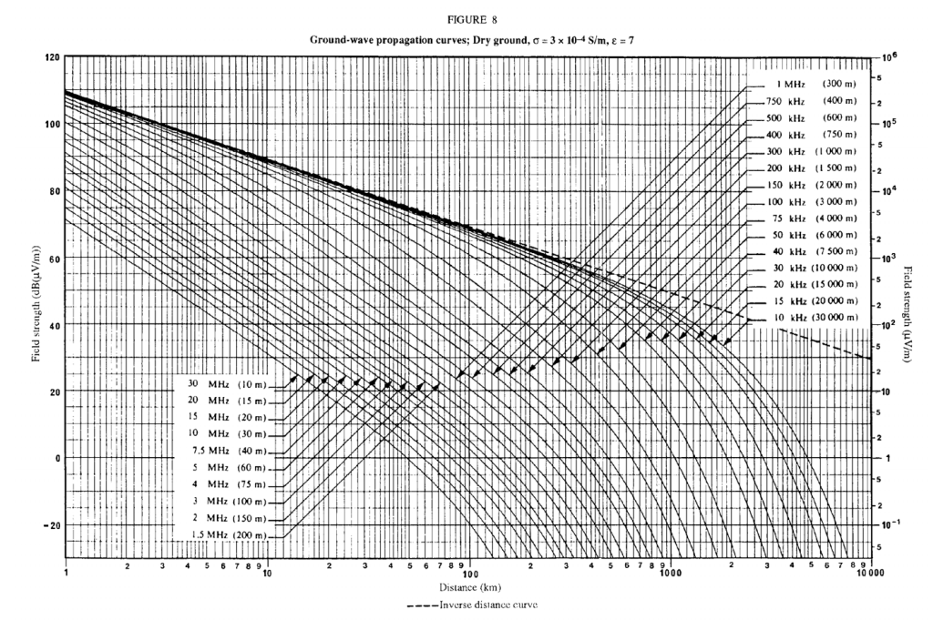 Whilst P.368-9 publishes a set of graphs like the one above for a limited set of grounds, ITU-R also publishes the program (GRWAVE.EXE) which can be used to calculate values for the user’s choice of ground and that is what was used for this article. The graph above is for a vertical monopole over ground with 1000W radiated, the antenna has directivity of 3, and the dashed line (inverse distance curve) is the field strength for a lossless ground (PEC). This can be verified with a spot calculation at 1km. Continue reading Polarisation of man made noise