This article discusses adding a second synchronous AC generator in parallel with a running synchronous AC generator.
For explanation, a simple context is used, two identical diesel engine driven generators with governed speed, no droop compensation, otherwise largely manual control, simple equivalent circuit of the machines. The complexity of other factors like harmonic currents etc are not discussed.
The simple model is useful as it underlies practical machines and is a good configuration to introduce the main principles of the operation.
To avoid typos, some of the text uses Python formatting of complex numbers.
Prerequisites for paralleling three phase synchronous generators
Prerequisites for paralleling three phase machines are:
- same phase sequence (eg both A-B-C);
- nearly the same voltage; and
- nearly the same frequency, and eventually same phase.
(1) does not apply to a single phase machine. (1) is resolved at the time of wiring up the machines and circuit breakers used to connect them to the bus. Unless changes have been made to machines or wiring, sequence should not need to be checked. After any reconfiguration or wiring changes phase sequence should be checked by a competent person.
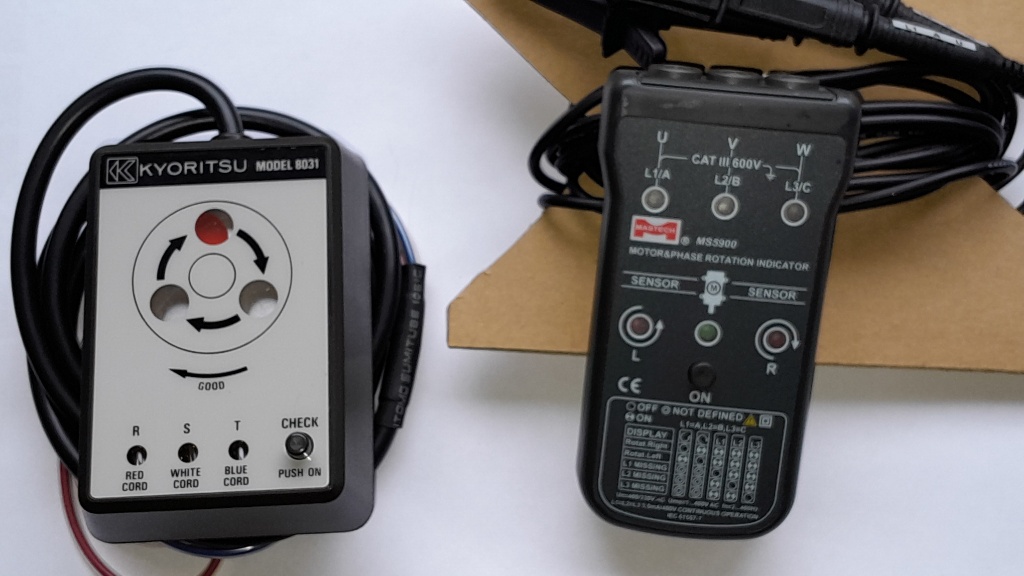
Phase sequence is checked using an instrument like one of these above. The left one is a small three phase motor, the right one is electronic and shows sequence with an LED.
Dot product of two phasors means the product of their magnitudes times the cosine of the phase difference, often calculated as \(V \cdot \overline{I}\) or V x I* to mean voltage times the complex conjugate of current.
The importance of (1) cannot be overstated, if the phase sequence is wrong, connection two machines together effectively short circuits at least part of them through the equivalent source impedance. Very large currents may flow, mechanical damage may occur (damaged crankshafts, engine bearings, alternator bearings, alternator laminations etc if bearings shatter… just don’t do it).
(2) and (3) are the substance of the process and will be explained in more detail.
Let’s clarify some terms and nomenclature
Unless stated otherwise, quantities should be taken as RMS, possibly with a non-zero phase angle.
Apparent Power (S) in an AC circuit is V * I in units of VoltAmps (VA), it is simply |V|*|I|.
Real Power (P) in an AC circuit is |V|*| I| *PF in units of watts (W), it it the real part of the dot product of voltage and current phasors.
Reactive Power (Q) in an AC circuit is |V|*|I|*(1-PF^2)^0.5 in units of VoltAmpsReactive (VAr), it it the imaginary part of the dot product of voltage and current phasors. Convention is that Q into an inductive load is +ve, and -ve Q signifies a capacitive load.
Power used without further qualification in this article means Real Power.
Load Power Factor is the cosine of the phase angle of current wrt voltage or PF=P/S, it is assumed current lags voltage. Sometimes -ve power factor is used to mean that current leads, an unusual condition, often prohibited as it can mean that a leading load can raise the bus voltage. That said, it is easy to unintentionally make a generator into a leading load, more later.
Simplified equivalent circuit of a synchronous generator
Equivalent source impedance
An imperfection of real world generators is that the terminal voltage is dependent on output current. The native generator inherently has some Thevenin output impedance, and a simple model is a Thevenin source equal to the no load voltage, and a series impedance that is usually dominated by the synchronous reactance.
This equivalent source impedance is very important parameter relevant to finding the magnitude and phase of current from a synchronous generator on an infinite bus, or on an island with one or more other synchronous generators.
It is common practice to specify internal impedance in pu or per unit (like per cent means per 100, per unit means per 1). An impedance of 0.1 pu means that if rated current flows, the impedance will produce a voltage drop of 0.1 (or 10%) of the rated voltage.
Equivalent source voltage
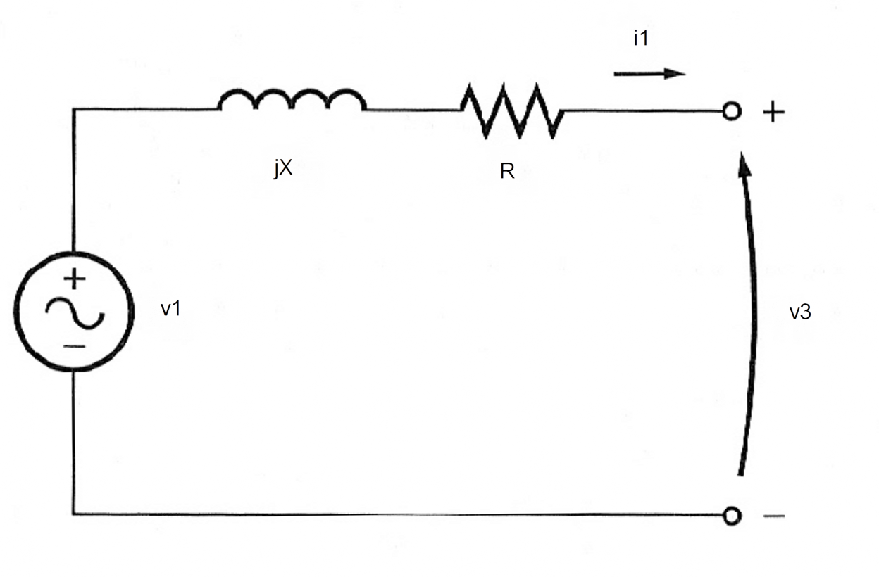
Above is a simplified equivalent circuit of the output side of a single phase synchronous generator (the input field circuit is not shown.) R -s the AC resistance of the armature winding (often taken to be 1.6 times its DC resistance due to skin effect), X is the sum of armature leakage and armature reaction (the latter is usually much larger).
A simple model of a synchronous generator without any form of voltage regulation is that the Thevenin equivalent voltage (or no load voltage) v1 is proportional to field current, and terminal voltage under load v3 will be lower as a result of current flow through the equivalent source impedance R+jX discussed earlier. We can calculate v1 from current i1 and source impedance Zs: \(v_1=v_3+i_1 Z_s\) noting that v1, v3, I1and Zs are complex quantities (magnitude and phase).
When two or more generators are in parallel, the unloaded voltage becomes very important is determining the magnitude and distribution of the reactive component of current.
Frequency
The frequency of the output of a synchronous generator is proportional to rotational speed \(f=\frac{NP}{60}\) where N is rotational speed in RPM and P is the number of pole pairs. For example, a machine with 4 pole pairs running at 750RPM generates 50Hz AC.
A simple widely used case is that the prime mover includes a proportional control to govern the rotational speed, and since output frequency is proportional to the rotational speed, so it is convenient to consider rotational speed in terms of frequency.
So where frequency is controlled by a proportional or P controller, and the energy input is proportional to the difference between the no load frequency (SV) and actual frequency (PV), \(f=f_0+{d_f} p\). This behavior can be used to control the sharing of power between two parallel synchronous generators.
An example
The example scenario is two identical machines, one running taking 100% of the load, and the second one is to be synchronised to the first, connected to the bus, and some load transferred to it.
Key parameters:
- f 50Hz
- S 20kVA
- PF 0.9
- rdf -0.0001111Hz/W
- rdv 0.1152+2.016jΩ
- load 10kVA @ PF 0.9
- before ACB close, f1=50Hz, f2=50.1Hz.
At ACB close
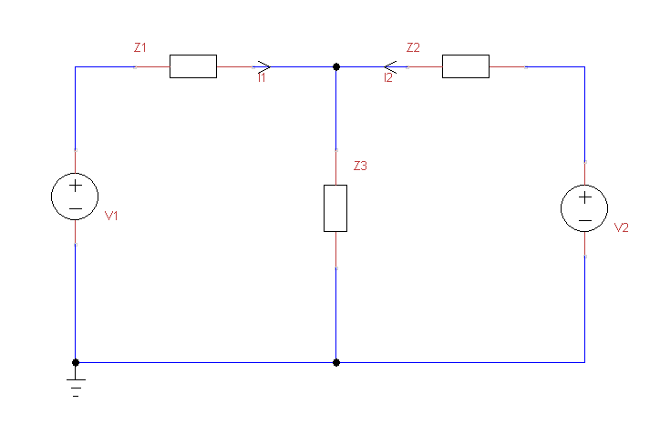
We can draw a schematic of the system after the second machine is connected to the bus.
When the ACB is closed connecting the incoming machine to the bus, its frequency can be thought of as locked to the bus frequency. In an ‘infinite’ bus, bus frequency is unaffected by the new generator, but in the example configuration, bus frequency is greater than it was and the actual frequency depends on the power sharing of the two generators.
It is often explained that once electrically coupled, the to generators act just like they are mechanically coupled. That is not strictly true, in each one the angle between the rotor and terminal voltage varies with power, and internal impedance.
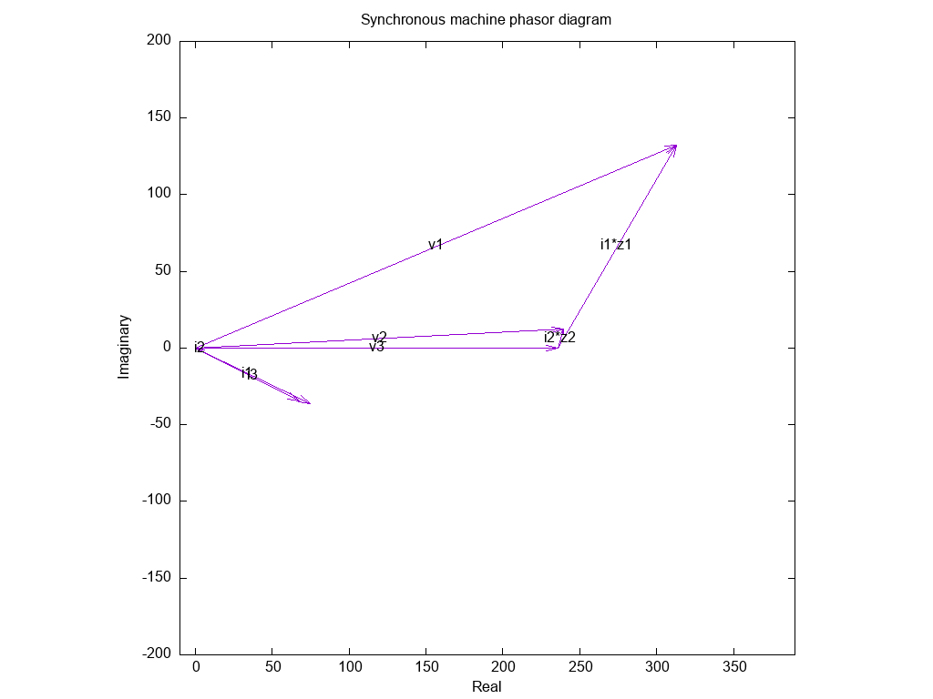
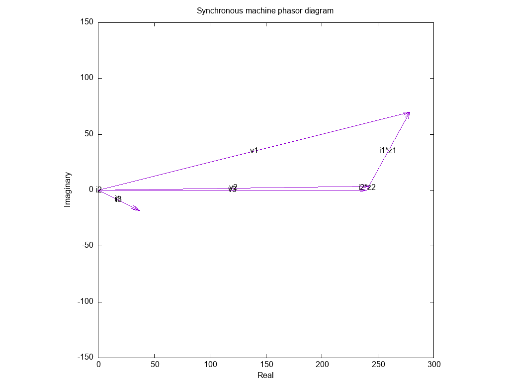
Above is a phasor diagram of two machines of the type discussed in parallel. This is just after ACB closure, and they are not well adjusted in this case to allow visibility of the various phasors.
The phase reference is the bus voltage v3, and one can note that i3 lags v3 by 26°, a consequence of the specified load PF=0.9.
Note that i1 is not exactly in phase with i2 which indicates less than perfect sharing of reactive current / power. This leads to the same angle between i1*zs1 and i2*zs2.
Most power (92%) is carried by the outgoing machine (#1) which is a little high as an initial condition on ACB close.
Above is a phasor diagram of ideal sharing at bus close. P and Q are both shared 95%/5%, the i1, i2, i3 phasors are inline, the Zs phasors are inline.
Power output of a machine is approximately proportional to the sine of the angle between EMF (eg v1) and terminal voltage (eg V3), this is known as the power angle or load angle of the synchronous machine. (See Synchronous machine power formula.) This angle will vary as power is transferred from one machine to another, and it may oscillate over hopefully a small range with load transients and rotors accelerating / decelerating. The phase of the rotor is related to the power angle, and it can be seen that the rotors are not truly in lockstep, but whilst rotating at the same average speed, there are small differences in speed to permit the change of the power angle as needed.
Coordinated adjustment of frequency and voltage are required to transfer load and manage reactive component of current
Frequency control / adjustment
From the above, we can calculate f0 for machine #1 carrying the entire load, \(f_0=f+{d_f} p\) giving f01=51.0Hz.
It is best when bring a second machine online that it carries a very small part of the power to minimise transients which might be disruptive or even cause damage.
So, let’s calculate the f0 for machine#2 so that when the circuit breaker (ACB) is closed to connect it to the bus, that it supplies say 2% of the power:
\(f_{0_2}=(sh_2)*(-rdf_1*s_3.real-rdf_2*s_3.real)+rdf_2*s_3.real+f_{0_1}\)and we get that f02 should be 50.09Hz. You would set the speed on machine #2 so the synchroscope rotates a full circle in about 10s.
Setting the incoming speed too low risks motoring the incoming set which confuses current measurements with basic instrumentation. Setting it too high risks a bigger transient, worsened by the fact that time to respond, press the button and close the ACB is more critical. Common practice is a beat period of about 10s, and press the button as the synchroscope rotates clockwise through the 11 o’clock position… these work in combination.
Under those conditions, the no load voltage of machine #2 should be very very close to the load voltage at the moment, so close that to use the actual load voltage at the time is sufficiently accurate, we will assume that the load volage v3 is 240V.
When the ACB is closed, the machines will both run at exactly the same (speed) frequency, and it will now be 50.05Hz (a result of the new power sharing arrangement).
Now to transfer more of the power to machine #2, frequency f01 needs to be decreased and f02 needs to be increased. This should be done incrementally keeping the actual frequency f within acceptable limits of 50Hz, say between 49.5 and 50.5Hz.
Realise that raising setting f01 does not raise the frequency to that value, you are raising the Set Value (SV) in a proportional control loop, and the Process Value (PV) or actual speed will increase by some amount, the prime mover will take more load and it will stabilise at some speed (PV) below SV proportional to the power input.
If the objective is to load share equally, then stop that process when the power supplied by each machine is equal.
If the objective is to take machine #1 offline (say for maintenance), continue adjusting f01 and f02 until the power supplied by machine #1 is say 5% of the load power and there is no circulating reactive current, then open its ACB to remove it from the bus. Be careful not to go too far and make machine #1 a motor (which is indicated by its current increasing with a decrease in f01).
Some control panels allow designation of the current operation as taking a machine offline, and when current falls sufficiently, it will automatically open the applicable ACB.
Voltage control / adjustment
The open circuit voltage (EMF) of a synchronous generator is proportional to the field current… up to the onset of magnetic saturation.
As the load is increased on a machine, the EMF needs to be increased to offset the voltage drop in the source impedance so as to maintain the desired bus voltage. (This may be done by an Automatic Voltage Regulator (AVR) but an AVR is not used in this article.)
There are a range of techniques for automatic regulation of the voltage of a synchronous generator, and what works for a stand alone generator may not usually work when two such machines are paralleled.
Let’s deal with the simpler case where field current manually adjusted to adjust the EMF of the generator.
A difference in the EMF of two paralleled generators may drive a current between the machines, a circulating current. Because of the nature of the equivalent source impedance discussed earlier, circulating current will tend to be highly reactive. Circulating current is undesirable, it increases R losses in the armature winding and may be sufficient to trip overcurrent protection and so limit the power available from a machine.
Circulating current is controlled by careful adjustment of the EMF of each generator, obtaining the desired loaded output voltage and with acceptably low circulating current.
As load power is shifted from machine #1 to machine #2, the EMF of machine #1 needs to be reduced and machine #1 increased.
We can calculate at at full load (just prior to ACB close), v1=287V, and that at 50% sharing, v1=v2=263V. If almost all the load is transferred to machine #2, v2 must be raised to 287 and of course v1 reduced to almost 240V so as to obtain v3=240V.
These voltage adjustments must be coordinated with the sifting of real power using the frequency controls discussed above.
The primary controls are:
- frequency to share real power whilst maintaining the required bus frequency; and
- voltage to share reactive power whilst maintaining the required bus voltage.
There is some interaction of the two controls, they are not independent.
Solution of an arbitrary configuration
We can draw a schematic of the system after the second machine is connected to the bus.
We can solve this network by mesh currents, let’s write the mesh equations.
\(v_1=(z_1+z_3)*i_1 +z_3*i_2\\v_2=z_3*i_1 +(z_2+z_3)*i_2\\\\\)
This is a system of 2 linear simultaneous equations in 2 unknowns. In matrix notation
\(\begin{vmatrix}i_1\\i_2 \end{vmatrix}=
\begin{vmatrix}
z_1+z_3 & z_3\\
z_3 & z_2+z_3
\end{vmatrix}^{-1} \times
\begin{vmatrix}v_1\\v_2\end{vmatrix}
\\\\\)
So, let’s solve an example:
- v1=(240+100)∠20°;
- v2=240∠0°; and
- z1: 1.152e-01+2.016e+00j, z2: 1.152e-01+2.016e+00j, z3: 5.184e+00+2.511e+00j.
The difference in magnitude and phase of the two sources will influence the sharing of real and reactive power.
To make this easier to understand, the complex quantities are adjusted after solving the equations using v3 as the phase reference.
The solution is:
- v1: 3.132e+02+1.324e+02j, v2: 2.397e+02+1.223e+01j, v3: 2.361e+02-2.842e-14j
- |v1|: 3.40000e+02, |v2|: 2.40000e+02, |v3|: 2.36144e+02
- i1: 6.765e+01-3.433e+01j, i2: 6.148e+00-1.407e+00j, i3: 7.379e+01-3.574e+01j
- |i1|: 7.58608e+01, |i2|: 6.30714e+00, |i3|: 8.33333e+01 s1: 1.59743e+04+8.10767e+03j, s2: 1.45187e+03+3.32218e+02j, s3: 0.77108e+04+8.57772e+03j
- pa1: 22.922°, pa2: 2.922°,ta1: 139.831°, ta2: 105.810°
Note the imaginary components of i, machine #1 is overexcited and it’s takes a larger share of reactive power, 94.5%, as opposed to 91.6% of the real power.
It can be challenging to properly apportion reactive power if the control panel does not include good instrumentation for reactive power, eg a centre zero VAr meter or centre zero Power Factor meter. Yes, you can get into a situation where reactive current of opposite polarity flows, quite easy with high Power Factor loads where just a small reactive imbalance causes opposite polarity reactive flow.
A final word of warning, some synchroscopes can be connected for only a very short period before they burn out, and if the panel has lights, review the mode (eg bright and dull) and the correct display at synchronisation… don’t mix them up… ever!
Conclusions
The distribution of power and reactive power is predictable using characteristics of the machines and a simple analytical model.
The common advice to set the incoming machine 0.1Hz higher than the bus, unloaded voltage equal to the bus, and to close as the synchroscope passes 11 o’clock is soundly based. It minimises risk of transients, violent rotor oscillation, torque damage to mechanical components , high circulating current which may trip overcurrent protection, etc. After ACB close, careful incremental changes to transfer the load to the incoming machine, keeping a close watch on bus voltage and frequency will lead to success.
Control panel instrumentation that shows the magnitude and direction of real power and reactive current or power on each machine and the load is useful for finding the way out of a messed up change where a machine may be driven to motoring or excessive circulating current.
The model does not support some of the magic recipes for changeover that one has heard from operators.
Suck it and see approach to syncronising machines may be quite dangerous, rotating machines possess a lot of energy and that energy can be disspated in destruction of infrastructure in just seconds.