Reworked for average ground type (σ=0.005, εr=3) …
A common scheme for narrow band match of an end fed high Z antenna discussed discussed the kind of matching network in the following figure.
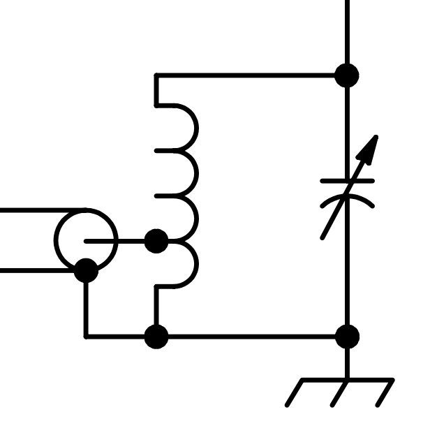
A common variant shows no capacitor… but for most loads, the capacitance is essential to its operation, even if it is incidental to the inductor or as often the case, supplied by the mounting arrangement of a vertical radiator tube to the mast. In any event, and adjustable capacitor may be a practical addition to help with matching under varying environmental factors.
This article is an expose on technique rather that a recommended antenna design.
The example antenna
The example antenna is a capacity hat loaded Marconi. An NEC-4.2 model characterised the antenna as:
- base fed with matching network to be discussed below;
- 25m vertical conductor;
- 2x 40m radial horizontal capacity had wires
- 8x 40m long elevated radials (0.1m); and
- average ground (σ=0.005, εr=3).
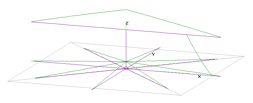
Above is a diagram of the antenna with current magnitude graphed in green.
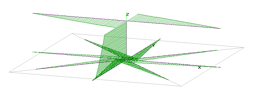
Above is a diagram of the antenna with current magnitude and phase graphed in green.
Radiator feed point impedance is 0.827Ω. Radiation efficiency of the radiator is 10.34% (implying radiation resistance Rr=0.827*0.134=111mΩ, structure efficiency is 86.0%. Radiation efficiency of the SYSTEM will be much lower.
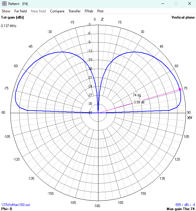
Above is the gain pattern plot, gain is about 9 dB down on a lossless antenna and of course, consistent with the radiator efficiency figure above.
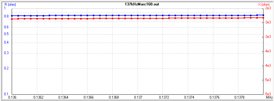
Above is a plot of base feed point impedance. As might be expected, R is a very small (+ve) value and X is a very large -ve value. This is a very challenging load to match efficiently.
Matching
So, let’s apply the matching network shown above.
Finding the matching network is not trivial, this is not something you would want to discover by suck it and see for this scenario.
A common scheme for narrow band match of an end fed high Z antenna gave a py script to help find the starting values. This article used an improved script to help prevent the optimiser roaming into badlands.
We need to make some assumptions and find the other parameters. Experience says the inductor needs to be very low loss, and it will be high inductance at this frequency. The prototype inductor is 300mm diameter, 5mm pitch, 125t of 3mm copper wire. The inductor is just over 600mm in length, and we might expect Q of just over 600.
TappedMatch.py v1.03 20240130 Owen Duffy

Inputs:
zl: (0.8277-2349j)
pitch: 0.00500 m, radius: 0.15000 m, turns: 125.00, length: 0.62500 m, Ql: 620, Qc: 5000

Results:
VSWR=1.00015, tap=1.227 (%), c1=242.50956 (pF)
Info: Lt=1.831e-03 (H), k=0.203
Yes, it took a few iterations to find the number of turns that would work.
SimNEC
Let’s take the NEC-4.2 results and those starting values to SimNEC.
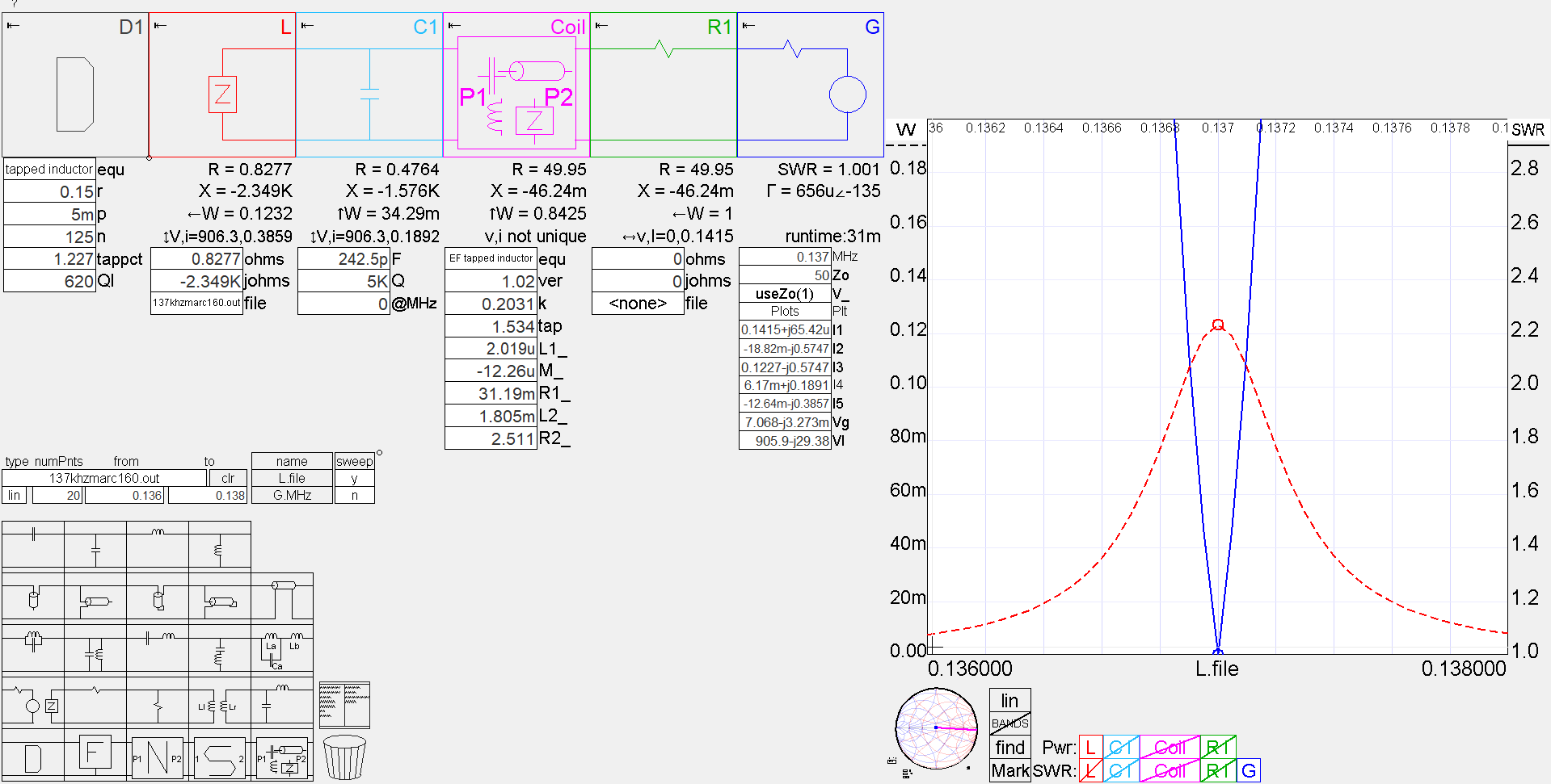
Above is a SimNEC model of such an arrangement.
The tapped coils is a uniform air cored solenoid of radius 150mm, pitch 5mm, 125t tapped at 1.227% (ie ~1.5t). Such a coil of 3mm copper should have unloaded Q around 620 @ 137kHz (from Hamwaves RF Inductance Calculator.)
C1 represents some additional capacitance to make the matching network adjustable.
Though it seems every ham thinks they can explain how this circuit works, there is nothing intuitive about the design of the tapped inductor.
Python script
The inductor design was assisted by a little python script which found the tap point and c1 for a given inductor, load, etc.
#!/usr/bin/env python
# coding: utf-8

import math
import cmath
from scipy.optimize import minimize
from scipy import constants
print('\nTappedMatch.py v1.03 20240130 Owen Duffy\n')

f=137e3
zl=0.8277-2349j

#network
qc=5000
ql=620
#tapped coil
p=0.005
r=0.15
n=125
#n=176.4

k=0
lt=0

def wcf(n,r,l):
#  print((1+math.pi*r/l)+1/(2.3004+1.622*l/r+0.4409*(l/r)**2),r,l)
  return constants.mu_0*n**2*r*(math.log(1+math.pi*r/l)+1/(2.3004+1.622*l/r+0.4409*(l/r)**2))

def vswr(args):
  global k,lt
  tap,c1=args
  lt=wcf(n,r,l)
  l1=wcf(n*tap,r,l*tap)
  l2=wcf(n*(1-tap),r,l*(1-tap))
  m=-(lt-l1-l2)/2
  k=abs(m)*(l1*l2)**-0.5;
  rlt=2*math.pi*f*lt/ql
  y=1/zl
  y=y+2*math.pi*f*c1*(1/qc+1j)
  zl2p=rlt*(1-tap)+2*math.pi*f*(l2-m)*1j
  z=1/y+zl2p
  y=1/z
  yl1p=1/(rlt*tap+2*math.pi*f*(l1-m)*1j)
  y=y+yl1p
  z=1/y
  zm=2*math.pi*f*m*1j
  z=z+zm
  y=1/z
  gamma=(z-50)/(z+50)
  rho=abs(gamma)
  vswr=(1+rho)/(1-rho)
  return vswr

l=n*p

#starting guess
tap=0.03
c1=10e-12

x0=[tap,c1]
bnds=((0.001,1),(0,None))
res=minimize(vswr,x0,method='Nelder-Mead',bounds=bnds)

print('Inputs:')
print("zl:",zl)

print('pitch: {:0.5f} m, radius: {:0.5f} m, turns: {:0.2f}, length: {:0.5f} m, Ql: {:0.0f}, Qc: {:0.0f}'.format(p,r,n,p*n,ql,qc))
print('\nResults:')
print('VSWR={:0.5f}, tap={:0.3f} (%), c1={:0.5f} (pF)'.format(res.fun,res.x[0]*100,res.x[1]*1e12))
print('Info: Lt={:0.3e} (H), k={:0.3f}\n'.format(lt,k))
print()
Above is the code, it elaborates the solution in small steps so that it is easier to understand. The script does not do much error checking, it will produce valid results on sane input.
If one plays with the Simsmith model, there is a solution with c1=0 for some load impedances, but in reality, the incidental capacitances mean that c1 is unlikely to ever be exactly zero.
A deep dive into the antenna SYSTEM
Let’s explore the currents in the matching network, no flywheels, no hand waving… just real numbers, well complex numbers actually.
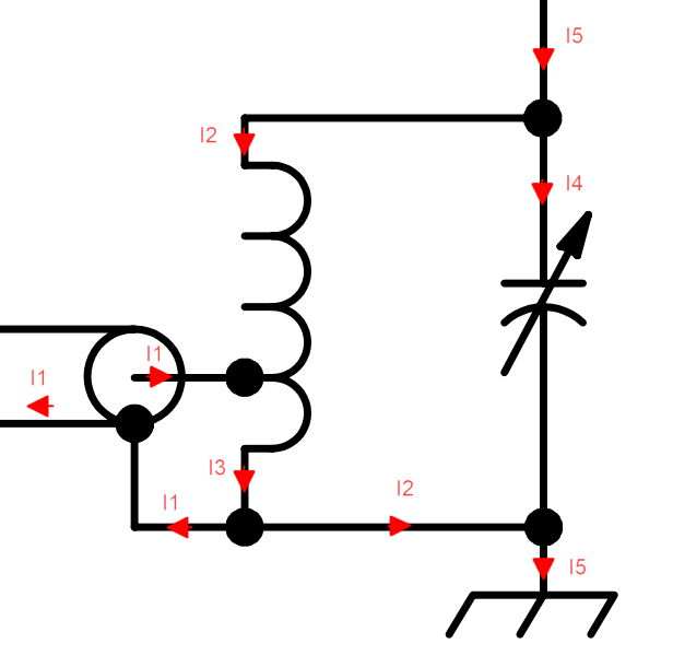
Above is the simplified schematic annotated with currents.
This model assumes there is zero common mode current on the coax, I1 is shown on the centre conductor and on the inside of the shield, but there is no current on the outside of the shield.
The SimNEC model is excited with 1W from the generator G.
Currents I1 to I5 are calculated in the SimNEC model, and are shown in a list under the G module. Also calculated are the terminal voltages for generator and load (Vg and Vl).
Some points to note:
- G sees an almost perfectly resistive load (the objective is 50+j0Ω), so the imaginary component of current I1 is much smaller than the real component;
- Vl is almost in phase with Vg, and much larger in magnitude;
- load impedance is highly capacitive (shortened Marconi), so load current would have a leading current, i5 is in the opposite direction, ie – load current (L.i in SimNEC) and hence has strongly lagging phase;
- I5 divides between the capacitor (I4) and upper section of the inductor (I2);
- capacitor current I4 is highly leading phase;
- upper section of the inductor current I2 is strongly lagging phase;
- lower section of the inductor current I3 is the sum of the current in the upper section and the current flowing in at the tap; and
- I3 is not a lot different to I2, the ‘tank’ is dominated by circulating current.
Dominated by circulating current means that there is much more current flowing in the tank circuit (L and C, I2 and I4) than flowing in the output terminal (I5).
Many of these points are the result of a high Q (low loss) tuned network.
So, the VSWR curve shows this is a high Q antenna SYSTEM, Q is around 100 compared to a half wave dipole at around 10-13. Tuning / matching will be quite critical.
The SimNEC model calculates loss in the matching network, 123mW is delivered to the radiator from 1W input (-9.1dB), and the radiator is 10.34% efficient (-9.86dB), so SYSTEM radiation efficiency is 1.27% or -18.96dB… giving a maximum gain of -3.99-9.1=-13.09dBi. With 1W input, EIRP is 49.1mW.
If a ham station with such an antenna SYSTEM was limited to say 1W EIRP, then a 21W output transmitter should achieve that limit. At that input power, the voltage across the matching inductor and capacitor would approach 6kVpk in the modelled scenario.
Validation
This is a desk study without implementation, there are no measurements.
If you were to build an antenna system for 137kHz, accurate measurement of the raw feed point impedance may be very challenging. In this case is was a resistance of around 0.8Ω in series with a reactance of 2349Ω (Q>2000). A VNA might give a reasonable estimate of the X part of Z, but accurate measurement of the R part in series with the expected X value will be challenging. Nevertheless, X gives a good indication of the amount of inductance in the matching network.
Measurement of Q of matching components is also challenging with Q again being very high.
One possibility is to measure field strength of the ground wave at sufficient distance to be confident that induction fields are insignificant, measure power input to the matching network and calculate system efficiency factoring in ground wave attenuation, see Reconciliation of transmitter power, EIRP, received signal strength, antenna factor, ground wave propagation etc @ 576kHz for relevant discussion.
At “sufficient distance”, field strength is proportional to 1/distance. Sufficient distance therefore is when field strength is proportional to 1/distance.
Measurements at distances from 5 to 20km would seem appropriate. Some authors state that far field conditions exist beyond a quarter wave from the antenna, but in practice these measurements do not settle down to \(E \propto \frac1r\) until \(r > 2 \lambda\).
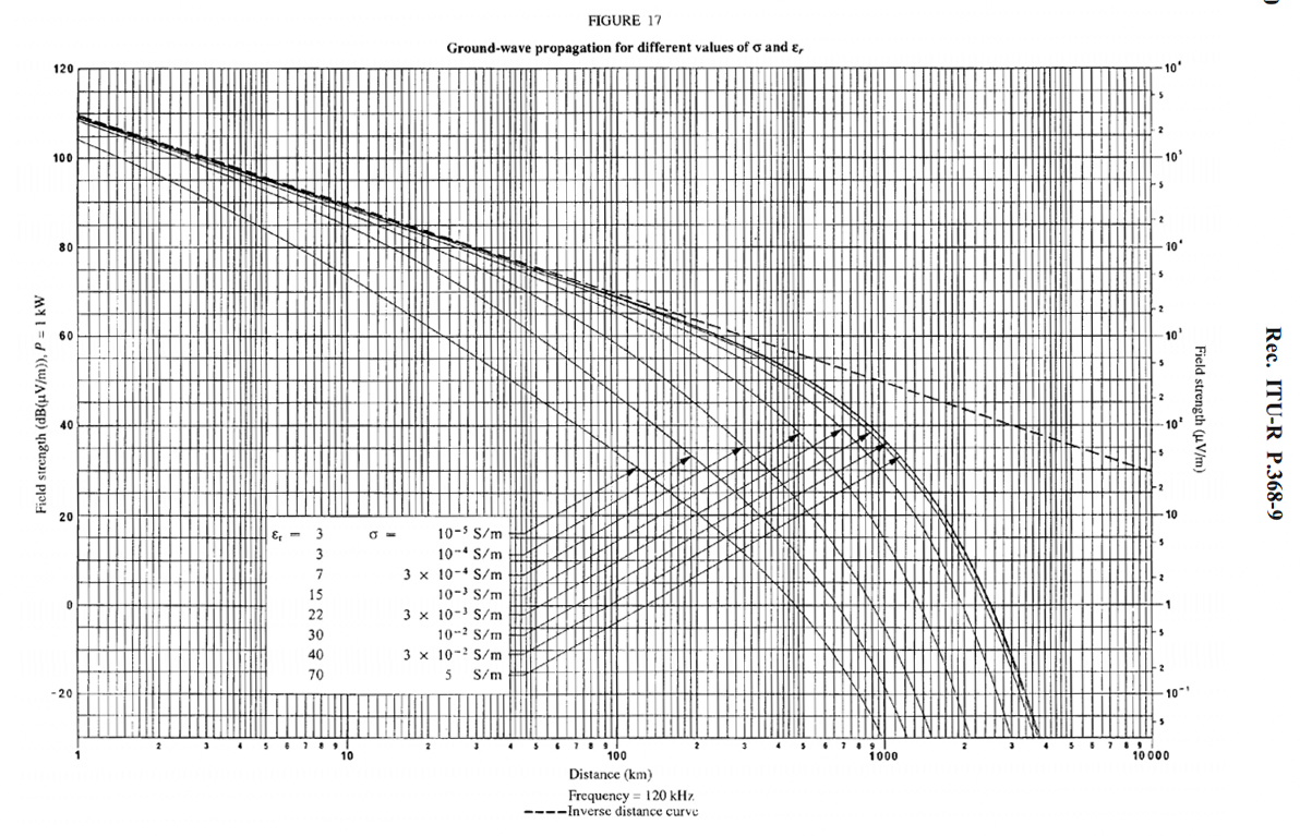
The graph above from ITU-R P.368-9 (now superceded) for a vertically polarised wave @ 120kHz suggests that the ground attenuation for common soil types at 5km is way less than 1dB, so field strength should be as calculated from Friis (free space) path loss and a further 0.1-0.2dB for ground attenuation.
Additional ground loss is dependent on soil type.
Note that ITU-R P.368 is based on 3kW EIRP (1kW into a lossless short monopole (directivity=3)).
It is unlikely that field strength measurement uncertainty is anywhere near as low a 0.1dB, and the additional ground loss could be ignored for distances 5-10km.
So this surface wave analysis can be used to infer antenna SYSTEM efficiency.
Using LFMFSmoothEarth.m
ITU publishes LFMFSmoothEarth.m to calculate a ITU-R P.368-10 updated version of the data shown in the graph from ITU-R P.368-9 above (ITU-R P.368-10 does not contain most graphs that were in ITU-R P.368-9.)
| Distance (km) | Fieldstrength (dBµV/m) |
| 5.00 | 60.71 |
| 6.00 | 59.12 |
| 7.00 | 57.77 |
| 8.00 | 56.60 |
| 9.00 | 55.56 |
| 10.00 | 54.64 |
| 11.00 | 53.80 |
| 12.00 | 53.03 |
| 13.00 | 52.32 |
| 14.00 | 51.67 |
| 15.00 | 51.06 |
| 16.00 | 50.49 |
| 17.00 | 49.95 |
| 18.00 | 49.44 |
| 19.00 | 48.96 |
| 20.00 | 48.51 |
Above is output from ITU’s LFMFSmoothEarth.m program for ‘average’ soil type (σ=0.005, εr=13) and 1W EIRP. The Field Strength column implements 1/r attenuation plus additional ground loss.
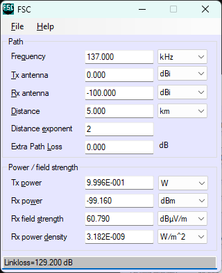
At 5km, Friis (free space) field strength with 1W EIRP is 60.79dBµV/m, so additional ground attenuation above is 60.79-60.71=0.08dB. An untuned small loop of practical size could have a gain around -100dBi, and the power received at 1W EIRP would be about -100dBm which could be measured with a receiver.
At 20km, additional ground attenuation is 0.24dB.
Optimisation
This example design is not optimised, it does not represent the ultimate outcome of dual purposing an existing 160m dipole.
Particularly, the inductor could be improved by changing its proportions, conductor size etc. Beware of close spaced turns, proximity effect my spoil the improvement sought.
The antenna structure might be improved with thicker conductors, more radials etc. Beware of buried radials, that might degrade radiation efficiency until there are a very large number of radials.
Conclusions
Shortened antennas have very low radiation resistance, low to very low loss resistance, and very large capacitive reactance, Q is of the order of thousands.
It may be very difficult to make accurate / complete / meaningful measurements of a shortened antenna.
Modelling is one method of getting insight into the likely feed point impedance for the purposes of design of an appropriate matching network.
Radiation efficiency of such an antenna system depends on a low loss matching network, and they are not trivial to improvise for a suck it and see approach to system tuning.
Field strength measurements in far field conditions are a possible way to evaluate actual system EIRP. Accuracy is adversely affected if there are significant induction fields present.
Calculation of path loss for EIRP evaluation depends on Friis (free space) path loss and ground attenuation, that at 137kHz at 5km, ground attenuation is of the order of 0.1dB.
References / links
- ITU-R 2022. Recommendation ITU-R P.368-10 (08/2022) Ground-wave propagation curves for frequencies between 10 kHz and 30 MHz. ITU-R.