nanoVNA – measure common mode choke – it is not all that hard!

It seems that lots of hams find measuring the impedance of a common mode choke a challenge… perhaps a result of online expert’s guidance?

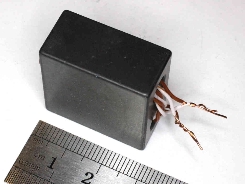
The example for explanation is a common and inexpensive 5943003801 (FT240-43) ferrite core.

Expectation

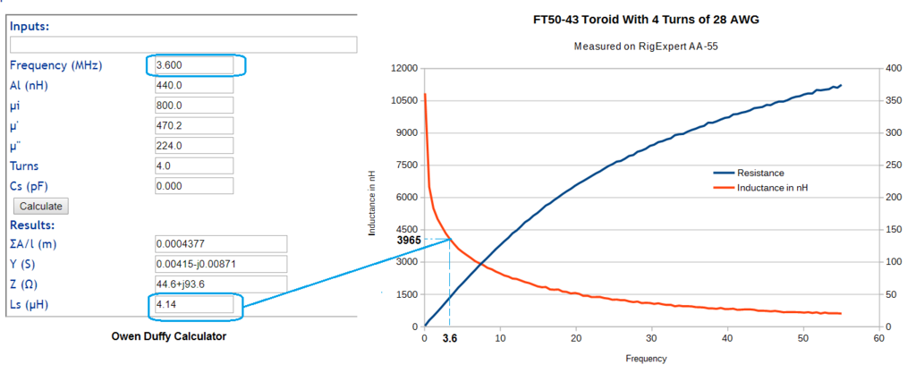
It helps to understand what we expect to measure.

See A method for estimating the impedance of a ferrite cored toroidal inductor at RF for an explanation.

Note that the model used is not suitable for cores of material and dimensions such that they exhibit dimensional resonance at the frequencies of interest.

Be aware that the tolerances of ferrite cores are quite wide, and characteristics are temperature sensitive, so we must not expect precision results.

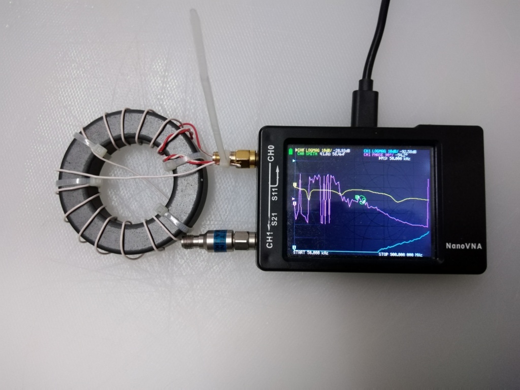
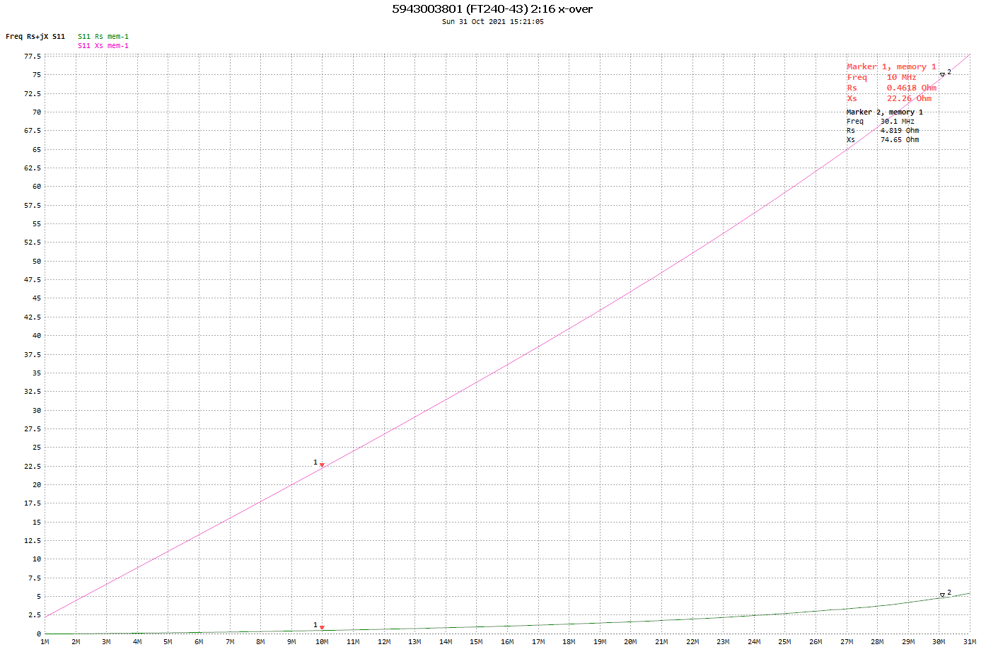
Above is a plot of the uncalibrated model of the expected inductor characteristic, it shows the type of response that is to be measured. The inductor is 11t wound on a Fair-rite 5943003801 (FT240-43) core in Reisert cross over style using 0.5mm insulated copper wire. Continue reading nanoVNA – measure common mode choke – it is not all that hard!

A simple Simsmith model for exploration of a 50Ω:200Ω transformer using a 2843009902 (BN43-7051) binocular ferrite core

EFHW-2843009902-43-2020-3-6kThis article applies the Simsmith model described at A simple Simsmith model for exploration of a common EFHW transformer design – 2t:14t to a ferrite cored 50Ω:200Ω transformer.

This article models the transformer on a nominal load, being \(Z_l=n^ 2 50 \;Ω\). Keep in mind that common applications of a 50Ω:200Ω transformer are not to 200Ω transformer loads, often antennas where the feed point impedance might vary quite widely, and performance of the transformer is quite sensitive to load impedance. The transformer is discussed here in a 50Ω:200Ω context.

Above is the prototype transformer using a 2843009902 (BN43-7051) binocular #43 ferrite core, the output terminals are shorted here, and total leakage inductance measured from one twisted connection to the other. Continue reading A simple Simsmith model for exploration of a 50Ω:200Ω transformer using a 2843009902 (BN43-7051) binocular ferrite core

A simple Simsmith model for exploration of a common EFHW transformer design – 2t:14t

This article describes a Simsmith model for an EFHW transformer using a popular design as an example.

This article models the transformer on a nominal load, being \(Z_l=n^ 2 50 \;Ω\). Real EFHW antennas operated at their fundamental resonance and harmonics are not that simple, so keep in mind that this level of design is but a pre-cursor to building a prototype and measurement and tuning with a real antenna.

Above is the prototype transformer measured using a nanoVNA, the measurement is of the inductance at the primary terminals with the secondary short circuited. Continue reading A simple Simsmith model for exploration of a common EFHW transformer design – 2t:14t

A simple Simsmith model for exploration of a common EFHW transformer design – 2t:16t

This article describes a Simsmith model for an EFHW transformer using a popular design as an example.

This article models the transformer on a nominal load, being \(Z_l=n^ 2 50 \;Ω\). Real EFHW antennas operated at their fundamental resonance and harmonics are not that simple, so keep in mind that this level of design is but a pre-cursor to building a prototype and measurement and tuning with a real antenna.

The prototype transformer follows the very popular design of a 2:16 turns transformer with the 2t primary twisted over the lowest 2t of the secondary, and the winding distributed in the Reisert style cross over configuration.

Above is a plot of the equivalent series impedance of the prototype transformer with short circuit secondary calculated from s11 measured with a nanoVNA from 1-31MHz. Note that it is almost entirely reactive, and the reactance is almost proportional to frequency suggesting close to a constant inductance. Continue reading A simple Simsmith model for exploration of a common EFHW transformer design – 2t:16t

Yet another ferrite toroid calculator – but is it any good?

In a recent online thread, a ‘new’ online calculator was touted:  https://miguelvaca.github.io/vk3cpu/toroid.html .

References without any qualification surely imply a recommendation.

In the same thread, Roger Need compared his measurement of a FT50-43 with Calculate ferrite cored inductor (from Al) (one of a set of related calculators), and Ferrite permeability interpolations.

Above, his calculation reconciles well with measurement at 3.6MHz. Continue reading Yet another ferrite toroid calculator – but is it any good?

Estimating characteristics of a sample of coax from dimensions and properties

On testing two wire line loss with an analyser / VNA – part 3 showed how to estimate two wire line characteristics from dimensions and an estimate of velocity factor. This article does the same for a coax example

To take an example, let’s use one posted online recently:

Stranded Tinned copper center conductor, 0.037″ od Solid, white dielectric (not foamed), 0.113″ od Od of jacket, 0.196″

The dimensions we are interested in are OD of dielectric, 2.97mm (0.113″) and OD of the inner conductor, 0.989mm (0.037″). A solid white dielectric (as opposed to translucent) is likely to be PTFE which has a velocity factor around 0.7 (in most PTFE cables) and we will assume a loss tangent of 1e-4 (typical of non-polar polymers). Continue reading Estimating characteristics of a sample of coax from dimensions and properties

On testing two wire line loss with an analyser / VNA – part 3

This article series shows how to measure matched line loss (MLL) of a section of two wire line using an analyser or VNA. The examples use the nanoVNA, a low end inexpensive VNA, but the technique is equally applicable to a good vector based antenna analyser of sufficient accuracy (and that can save s1p files).

On testing two wire line loss with an analyser / VNA – part 1

This article series shows a method for estimating matched line loss (MLL) of a section of two wire line based on physical measurements (Duffy 2011).

Above is a short piece of the line to be estimated. It is nominal 300Ω windowed TV ribbon. It has copper conductors, 7/0.25, spaced 7.5mm. The dielectric is assumed to be polyethylene… but later measurements suggest is has slightly higher loss than polyethylene. The test section length is 4.07m. Continue reading On testing two wire line loss with an analyser / VNA – part 3

On testing two wire line loss with an analyser / VNA – part 2

This article series shows how to measure matched line loss (MLL) of a section of two wire line using an analyser or VNA. The examples use the nanoVNA, a low end inexpensive VNA, but the technique is equally applicable to a good vector based antenna analyser of sufficient accuracy (and that can save s1p files).

On testing two wire line loss with an analyser / VNA – part 1

Above is a short piece of the line to be measured. It is nominal 300Ω windowed TV ribbon. It has copper conductors, 7/0.25, spaced 7.5mm. The dielectric is assumed to be polyethylene… but later measurements suggest is has slightly higher loss than polyethylene. The test section length is 4.07m. Continue reading On testing two wire line loss with an analyser / VNA – part 2

On testing two wire line loss with an analyser / VNA – part 1

This article series shows how to measure matched line loss (MLL) of a section of two wire line using an analyser or VNA. The examples use the nanoVNA, a low end inexpensive VNA, but the technique is equally applicable to a good vector based antenna analyser of sufficient accuracy.

Above is a short piece of the line to be measured. It is nominal 300Ω windowed TV ribbon. It has copper conductors, 7/0.25, spaced 7.5mm, though as can be seen the spacing is not perfectly uniform. The dielectric is assumed to be polyethylene… but later measurements suggest is has slightly higher loss than polyethylene. The test section length is 4.07m. Continue reading On testing two wire line loss with an analyser / VNA – part 1

Do I ‘need’ a masthead preamp to work satellites on 2m? – G/T vs G/Ta

A reader of Do I ‘need’ a masthead preamp to work satellites on 2m? – space noise scenario has written to say he does not like my comments on the hammy adaptation of G/T.

Above is an archived extract of a spreadsheet that was very popular in the ham community, both with antenna designers and sellers and end users (buyers / constructors). It shows a column entitled G/T which is actually the hammy calculation. The meaning possibly derives from (Bertelsmeier 1987), he used G/Ta.

Ta is commonly interpreted by hams to be Temperature – antenna. It is true that antennas have an intrinsic equivalent noise temperature, it relates to their loss and physical temperature and is typically a very small number. But as Bertelsmeier uses it, it is Temperature – ambient (or external), and that is how it is used in this article.

Let’s calculate the G/Ta statistic for the three scenarios in Do I ‘need’ a masthead preamp to work satellites on 2m? – space noise scenario.

Base scenario

Above is a calculation of the base scenario, G/T=-29.74dB/K.

Also shown in this screenshot is G/Ta=-23.98dB/K. Continue reading Do I ‘need’ a masthead preamp to work satellites on 2m? – G/T vs G/Ta