Does RBN give a reliable metric for comparing antennas? gave an example of signal strength measurement and the effect of fading over time.
This article goes into a little more depth on the subject using a further data capture of 600 measurements 10s apart.
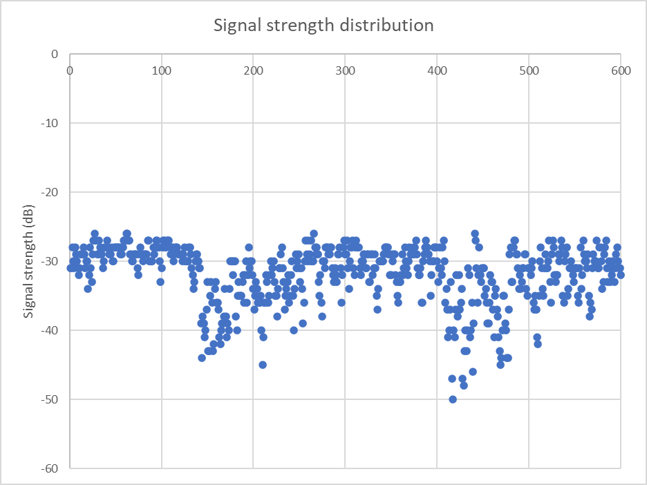
Above is a plot of signal strength of an 80m A1 Morse (CW) beacon measured in 20Hz bandwidth over 100min (a terrestrial path of length 105km).
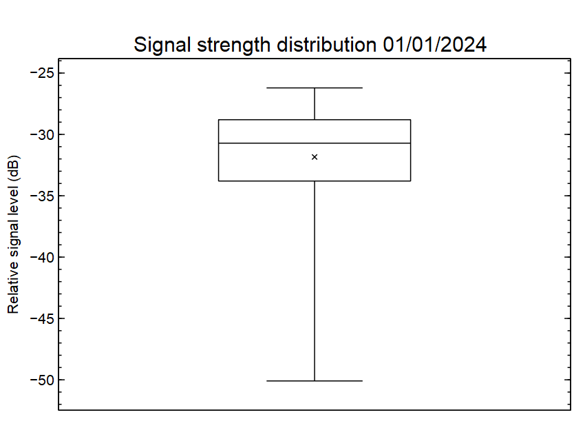
Above is a box plot of the data distribution. On this capture, values ranged from -50 to -26dB, a range of 24dB. 50% of observations are contained within the inter quartile range (IQR), 5dB. The mean (x in the box) is a little different to the median (horizontal line inside the box) hinting that it is a skewed distribution, and probably not a normal distribution.
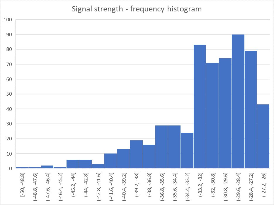
Above is a frequency histogram of the data, it does not resemble the bell shaped distribution of a Normal distribution.
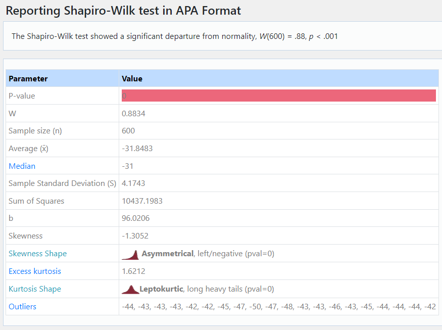
Above is a Shapiro-Wilk test for normality, the data fails is terribly.
Despite the distribution being not Normal, there is a tendency for people to apply statistical techniques that are based on Normal distribution, so let’s follow their lead.
Assuming Normal distribution
Two adjacent samples of 10 measurements were drawn randomly from the set of data to represent measurements that might be made comparing two antennas.
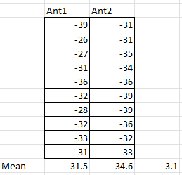
Above are the data sets drawn, and calculated means and the difference of the means. Does this mean Ant2 is 3.1dB better than Ant1?
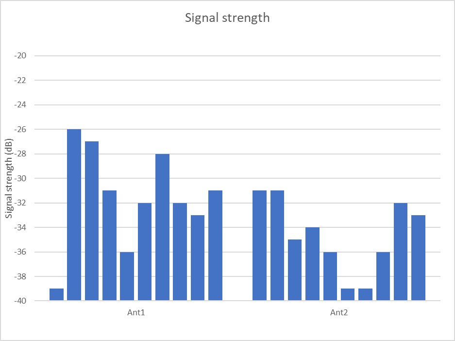
Above is a column chart of the two sample sets. Can you determine if one is better by eye? How much better?
Continuing with our assumption of Normality, we can apply Student’s t test to compare means of the two samples.
A test of the data assuming Normality and independent samples gives a 95% Confidence Interval of -0.731dB to 6.931dB for the estimate of the differences of the population means, and zero is in that range. In other words, we could not assert with 95% confidence that there was any difference between Ant1 and Ant2.
In fact
In fact Ant1 is the same as Ant2, any observed difference in the sample means in this case is entirely by chance given the variation in measurements.
To conclude there was simply 3.1dB difference in the population means would be naive. When you add the confidence interval to the sample means, it encompasses zero difference which is in fact true of the underlying system in this case… the difference in sample means is a result of chance.
Improving the result
Increasing the number of observations n improves accuracy as the sample means are more likely to be closer to the population means. Diminishing returns applies as n is increased.
Rounding of input data (eg to integer dB) adds statistical noise, degrading the result… but lots of tools supply measurement data rounded to whole dB.
Small n leads to a wide confidence interval and unless the difference in the sample means is very large, an inconclusive result.
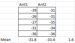
Here is an example where I use only the first five of each data set, and although the difference of the sample means is smaller, the 95% confidence interval of difference in population means is -5.885dB to 9.085dB… almost twice the width.
It is naive to rely solely on the difference in the sample means.
Experimental design
Better experimental design can give more useful results.
Noting that in the full dataset shown in the first graph, the first part is subject to less variation than later parts.
Selecting the first 100 observations and allocating the alternately to Ant1 and Ant2 simulates an experiment where measurements were made alternately using Ant1 and Ant2. This somewhat masks slower fading variation, not quite paired observations, but an improvement. (Paired observations would be even better if possible.)
For this scenario, the difference of the sample means is smaller at 0.06dB, the 95% confidence interval of difference in population means is -0.6596dB to 0.7796dB … much narrower and more convincing that there is probably no significant difference between Ant1 and Ant2.
But, the example data is not normally distributed
… and often / usually is not for this type of experiment. Nevertheless people use the data as if it was Normally distributed.