Category: Amateur Radio

Magnitude and phase of V2/V1 for a transmission line section ended with:

The quantities I2/V1 and V2/I1 can be more interesting in some applications.

This article discusses the quantity I2/V1 for a special case, a 90° transmission line section.

90° transmission line sections are often used as a splitter / combiner / impedance transformer for two nearly identical antennas. I say “nearly” because no two antennas are likely to be exactly identical. They are sometimes called phasing harnesses.

Above, an example. Continue reading Magnitude and phase of I2/V1 for a 90° transmission line section

Tuning electrical line length using phase of measured s21 – nanoVNA discussed the relationship between phase of s21 and the electrical length of a line section.

An interesting question is the magnitude and phase of the ratio V21 (V at port2 to V at port 1) in the presence of a standing wave.

At first you might answer that the phase difference is exactly that due to the electrical length of the transmission line section, the magnitude might be harder to guess.

There is a simple graphical solution on the Smith chart, yes it was designed to solve this problem.

Recall that the Smith chart is a polar plot of the complex reflection coefficient Γ, so when we plot an impedance point using the R and X scales, we are plotting a vector from the prime centre of the Smith chart, its length being |Γ|=ρ and angle being the angle of Γ.

The voltage at a point on the line is the sum of the forward and reflected waves, its relative magnitude is 1+Γ, known as the Transmission Coefficient. This vector is plotted from the R=0,X=0 point to the impedance of interest.

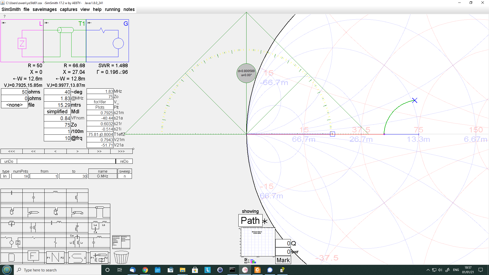
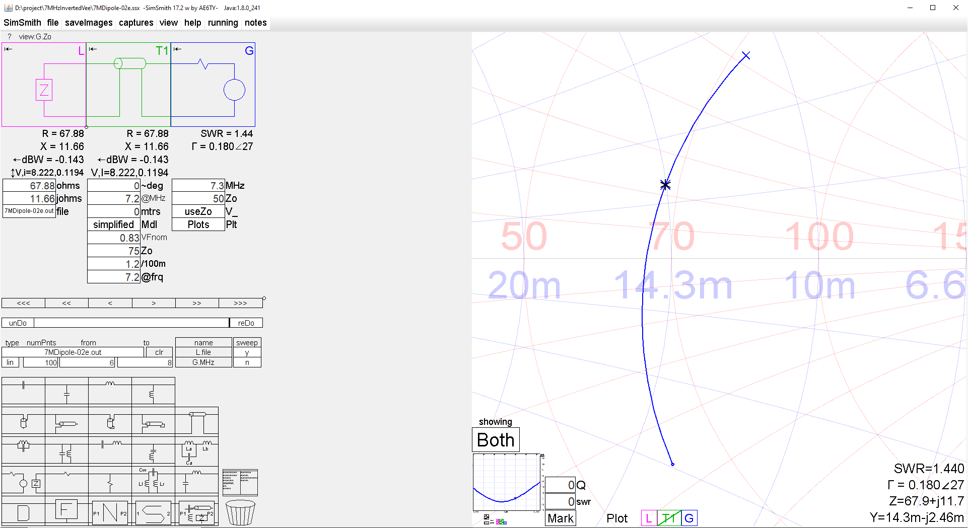
Lets look at the case of a 50+j0Ω load on a 75Ω line of length 40°.

We will start at the load end of the line, that is the way these problems are solved.

Above is a screenshot of the scenario from Simsmith. I have added a calibrated screen ruler to measure the Transmission Coefficient 1+Γ. 1+Γ=0.8∠0°.

Now lets look at the relationship at the other end of 1+Γ at that end.

From the screenshot, 1+Γ=0.99∠11.5°. Now recall that the relationship we noted above at the load end is 40° delayed from the source end, ie the phase is -40°. So the ratio \(V_{21}=\frac{V2}{V1}=\frac{0.8∠-40°}{0.99∠11.5°}=0.81∠-51.5°\). Keep in mind that although I used a screen ruler, this is still a graphical solution and accuracy is not as good as a calculation. In fact, calculation gives 0.7943∠-51.71°.

If you were to use a oscilloscope or vector voltmeter to measure the two voltages V1 and V2 and calculated V2/V1, you should get something very close to 0.8∠-52°.

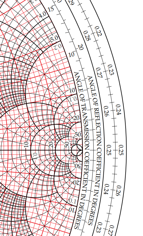
Recall that I said that the Smith chart was designed to solve this problem. I used a screen ruler to measure the 1+Γ vectors, but on a paper Smith chart you might use a protractor and ruler… but lets look at the inbuilt scales.

Note the innermost circular scale ANGLE OF TRANSMISSION COEFFICIENT IN DEGREES. The tick marks might look like they are at a strange angle, but they are for measuring the angle of 1+Γ vectors projected from R=0,X=0 to the scale. This scale can be used to measure the angle using only a ruler (or a piece of cotton and dividers for that matter).

The important finding in all of this is the the phase relationship between V2 and V1 under standing waves is not simply equal to the electrical length of the line.

A modified procedure can be followed to find I2/I1, an exercise left to the reader.

The quantities I2/V1 and V2/I1 can be more interesting in some applications.

Conclusions

The ratio V2/V1 can be found, it is not what many people might first guess and the solution goes to the heart of understanding transmission lines.

The nanoVNA has put a quite capable tool in the hands of many hams who do not (yet) understand transmission lines.

A recent online posting asked why phase of s21 of a desired 40° section of 75Ω matching / phasing line did not reconcile with other estimates of its electrical length.

Discussion

Let’s firstly review the meaning of s21.

Considering the two port network above, \(s_{21}=\frac{b_2}{a_1}\) where a and b are the voltages associated with incident and reflected travelling wave components. Implicit in the meaning of s parameters are the port reference impedances which in the case of the nanoVNA are nominally 50+j0Ω. Continue reading Tuning electrical line length using phase of measured s21 – nanoVNA

Hams often would like to know the impedance of an antenna at its feed point, sometimes for very sound reasons, and very often in pursuit of a specious goal.

One of the oft given suggestions is that it is convenient to measure through an integral number of electrical halfwaves of transmission line, since as everyone knows, impedance at the end of the line is repeated exactly every half wave towards the source.

Some even tell us that they cut their feed line lengths to exactly nλ/2 to facilitate this at implementation an into the future. So, lets take that idea and cut the feedline to the shortest nλ/2 that will reach the feed point 100m distant. The electrical length of a VF=0.83 feedline will need to be nλ/2 or 1080° at our nominal frequency of interest, 7.2MHz.

To explore the method, let’s use the modelled feed point impedance of a 40m Inverted V Dipole used in some recent articles.

The real feed point

Above is a Simsmith model of the feed point impedance, The blue line overlays the magenta line which is the locus of s11 from the NEC model. Continue reading On measuring antennas through integral halfwaves of transmission line

I have seen several online posts of hams citing measurement of phase of s11 as a figure of merit of a matched antenna system, indeed evidence of the resonance nirvana.

Let’s review the meaning of s11.

s11 is the complex reflection coefficient at the reference plane, usually wrt Zo=50+j0Ω.

If you were to measure the s11 looking into an ATU, you might adjust the ATU to minimise the magnitude of s11 (|s11|) which is also minimises VSWR. If you do a really really good job of adjustment, you might achieve around the noise floor of the instrument.

You can simulate this near perfect match by simply sweeping your 50Ω calibration load. Let’s do that and look at some relevant views.

Above, |s11| expressed in dB is very low, it is at the noise floor of the calibrated instrument, and it is very jittery… due to the relatively high contribution of noise. Continue reading On the measured phase of s11 in a matched system