Transmission line measurements – learning from failure

Introduction

A recent article questioned the accuracy of measurement of Matched Line Loss (MLL) for a modified commercial transmission line. The published results were less than half the loss of an equivalent line in air using copper conductors and lossless dielectric, when in fact there would be good reason to expect that the line modification would probably increase loss.

How do you avoid the pitfalls of using analysers and VNAs to measure line loss?

Lets walk through a simple exercise that you can try at home with a good one port analyser (or VNA). Measuring something that is totally unknown does not provide an external reference point for judging the reasonableness of the results, so will use something that is known to a fair extent,

Experiment

For this exercise, we will measure the Matched Line Loss (MLL) of a 6m length of uniform transmission line, RG58C/U cable, using an AIMUHF analyser. The AIM manual describes the method.

If you need to know the cable loss at other frequencies, enable the Return Loss display using the Setup menu and click Plot Parameters -> Return Loss and then do a regular scan of the cable over the desired frequency range with the far end of the cable open. Move the blue vertical cursor along the scan and the cable loss will be displayed on the right side of the graph for each frequency point

Note the one-way cable loss is numerically equal to one-half of the return loss. The return loss is the loss that the signal experiences in two passes, down and back along the open cable.

Our measurements will show that this is a naively simple explanation, and to take it literally as complete may lead to serious errors. Yes, it IS the equipment manual, but it is my experience that the designers of equipment, and writers of the manuals often show only a superficial knowledge of the relevant material.

Datasheet

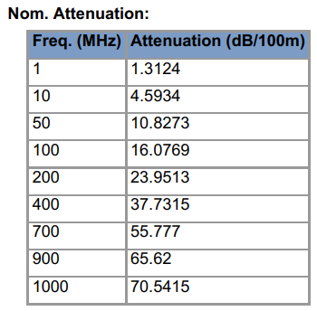
Above is an extract of the datasheet for Belden 8262 RG58C/U type cable, our test cable should have similar characteristics. Continue reading Transmission line measurements – learning from failure

VSWR meter trap for the unwary

From time to time one sees discussion online about consistency of ‘measured’ VSWR at different power levels (on the same instrument).

A question often asked is:

I tune up at 10W and achieve VSWR=1.5, and when I increase power to 100W, the VSWR increases. Which should I believe?

The first thing to note is that good antenna systems SHOULD be linear, VSWR should be independent of power, it is if the system IS linear.

For the most part they are linear, even though many antenna systems contain elements such as ferrite cored inductors that may exhibit some small level of non-linearity in ‘normal’ operation.

Non-linearity caused by for instance saturation of magnetic materials, loss of permeability where the temperature of ferrite cores reaches Curie point, arcing of capacitors or other insulating materials is NOT normal linear operation of a GOOD antenna system. If high indicated VSWR at high power is caused by any of these effects, it is flagging a problem that requires attention.

That said, a significant non-linear element may be the VSWR meter itself.

A common, if not most common way to make these meters is to use a half wave detector to convert the direction coupler RF outputs into DC to drive an ordinary moving coil meter. These meters commonly assume that the detector DC output voltage is exactly proportional to the RF input voltage.

Lets look at the accuracy of that process.

Above is a plot of the detector output vs RF input voltage for a commercial 200W VSWR meter. The measurements cover input power from 10 to 100W.
Continue reading VSWR meter trap for the unwary

WSPR for A/B tests – a discussion – part 4

Continuing from WSPR for A/B tests – a discussion – part 3.

Regression techniques

Another technique for exploring the relationship between paired variables is a regression model. In the case of these experiments, a simple model that is a good candidate is that SNR_B=m*SNR_A+b, a simple linear regression. A simple  solution is to find m and b to minimise the sum of squares of errors between the predicted SNR_B and measured SNR_B.

Above is a frequency distribution of data extracted from a month studied in 2011. There are almost half a million spots on 40m contributing to this analysis, so it covers a wide range of propagation conditions during the month, and includes all stations spotted by all stations. Continue reading WSPR for A/B tests – a discussion – part 4

WSPR for A/B tests – a discussion – part 3

Continuing from WSPR for A/B tests – a discussion – part 2.

Other tests for normality

Above is a frequency histogram of the experiment log.

I used the Shapiro-Wilks test for normality earlier, it is one of many, and they each have strengths and weakness, or sensitivities to some types of non-normality if you like.

Chi-squared test for normality

We could shop for a normality test that is less bothered by the rounded data. Pearson’s Chi-squared test is an obvious choice as it compares the frequency histogram on chosen classes with the expected distribution if the data was normal. So if we cleverly make the classes 1dB, we might have a test that is not sensitive to the rounded data. Continue reading WSPR for A/B tests – a discussion – part 3

Adjusting modulation level on FM mobiles etc.

One frequently hears FM radios on the VHF bands that high or low in modulation level which exacerbates the problem of copying stations whilst mobile.

The defence often given is that it is so hard to measure frequency modulation, that it take an expensive deviation meter and they are scarce.

This article explains how to make accurate measurements using equipment often found around ham shacks, and could certainly be cobbled together from the resources of a few ham shacks. The figures and example given apply to nominal 25kHz channeled radios, adjustments are need for narrow channel radios.

There are three steps where calibration is progressively transferred through a measurement chain:

  1. calibrate a modulator (an ordinary FM transmitter);
  2. calibrate a demodulator (an ordinary FM receiver) using the calibrated modulator;
  3. measure the unknown transmitter using the calibrated modulator.

Measurement

1. Calibrate a modulator

The usual method of calibrating a modulator is to use the spectral properties of an FM signal.

One could use a spectrum analyser to find the calibration point, adjusting the modulation level and  detecting the null of the carrier or sidebands according to the Bessel function.

Since the instrumentation is used to detect the null of a carrier or sideband component, and the null is very sensitive, a narrow band receiver can be used for the calibration procedure.

A practical approach

This is a procedure to calibrate a frequency modulator at a single modulating frequency using an SSB receiver to detect the first carrier zero.

  1. Prepare to modulate the carrier source (the transmitter) with a 1kHz (exactly) sine wave modulation source, adjust to zero modulation level and key the transmitter up.
  2. Couple a small amount of the carrier to an SSB receiver and tune in the carrier to a beat note of about 800 Hz.
  3. Slowly increase the modulation until you hear the carrier beat disappear. Carefully find this null position of the carrier beat note. Note that you will also hear one or more sidebands when the modulation is applied, ignore these and just listen for the null of the carrier.

The modulation index is now 2.4, and therefore the deviation is 2.4kHz.

The technique is very sensitive and very accurate, and error will mostly be attributed to the accuracy of the modulating frequency.

You have read about it, click to listen to a demonstration. This demonstration uses an SSB receiver with a 3.5kHz IF bandwidth, but I have used the technique with receivers with a 10kHz IF bandwidth, you just hear more of the sidebands, but concentrate on the carrier beat and null it out. The test receiver could be a high quality communications receiver or a scanner with a BFO. You could sample the modulated signal at the carrier frequency, or by sniffing some signal from the IF of a super-heterodyne receiver.

2. Calibrating a demodulator

Having calibrated a modulator, we can set a receiver up to demodulate that signal and calibrate its output voltage against the known deviation of the source.

Above, an oscilloscope is connected to the receiver output and the volume control is adjusted until the peak voltage is 2.4 divisions, corresponding to peak deviation of 2.4kHz. Continue reading Adjusting modulation level on FM mobiles etc.

WSPR for A/B tests – a discussion – part 2

Continuing from WSPR for A/B tests – a discussion – part 1.

Above is a frequency histogram of the experiment log.

Approximately…

The histogram uses 1dB intervals for the bars, so it chunks the data into discrete bands, and that hides an important issue with WSPR SNR data, its granularity is 1dB, so it is a very coarse measure given the spread of the data.

Lets compare the probability distribution of the measured difference data with an ideal normal distribution.

Above is a quantile-quantile (Q-Q) plot of the raw data and an ideal response with the same standard deviation as the raw data. The data is for 4508 points, so these dots each typically represent a large number of observations, more so in the middle region. Continue reading WSPR for A/B tests – a discussion – part 2

WSPR for A/B tests – a discussion – part 1

The WSPR  User Manual sets out the purpose of WSPR:

The WSPR software is designed for probing potential radio propagation paths using low power beacon-like transmissions.

Though that talks about measuring radio paths, it is often used to compare transmitters or receivers over radio paths.

WSPR SNR measurements include the end to end radio path, which on some bands is highly variable, so using WSPR reported SNR values to compare two transmitters can be quite challenging.

A/B tests

We are all familiar with ad-hoc tests where a station might switch between two antennas and ask for comparative reports from receiving stations. At time when the radio path characteristics change greatly, changes in transmitter are often masked or confused by path variation.

Of course some practitioners will conduct several so-called A/B changes, perhaps as many as five and someone (receiver or transmitter) makes an informal judgement of the central tendency of the observations. The observations might be given in quite subjective terms, or in quantitative terms, possibly from an S meter of unknown calibration.

Normal distribution

Repeated measurements of the same thing, or same type of thing (eg 10 measurements of 1 new dry cell, or one measurement each of 10 new dry cells) tend to yield a set of slightly different observations.

For a lot of common physical things, the distribution of repeated measurements follows a bell shaped probability curve.

Most things that we repeatedly measure will return slightly different results from observation to observation due to various contributions in an imperfect world.

Above is a plot of the probability distribution of a normally distributed random variable with mean=1 and variance=1 (standard deviation=1). Continue reading WSPR for A/B tests – a discussion – part 1

Checkout of SimSmith v16.3 – spot check of transmission line database – further discussion

The article Checkout of SimSmith v16.3 – spot check of transmission line database raises an issue with SimSmith’s modelling of transmission lines.

The case chosen was Belden 8216, a RG174 type line with silver clad steel stranded inner conductor.

Fully developed skin effect

Most practical transmission lines used for HF and above have fully developed skin effect above some frequency, and are well represented by the loss model MLL=k1*f^0.5+k2*f. For an RLGC model, the R is given by the first term and with fully developed skin effect, it is proportional to square root of f. The loss of good dielectrics is usually simply proportional to f and indicated by the second term.

Under this model, L and C are independent of frequency.

Many calculators use this model, and it works fine where skin effect is fully, or even well developed. The model coefficients are commonly discovered by performing a regression on measured matched loss at a range of frequencies, and the quality of the regression fit is a good indicator of the quality of the model for that particular line. Continue reading Checkout of SimSmith v16.3 – spot check of transmission line database – further discussion