CNC6040 router project – spindle speed linearisation

A known issue with the common CNC6040 router and similar devices is very poor calibration / linearity of the spindle motor response to gcode Sx commands.

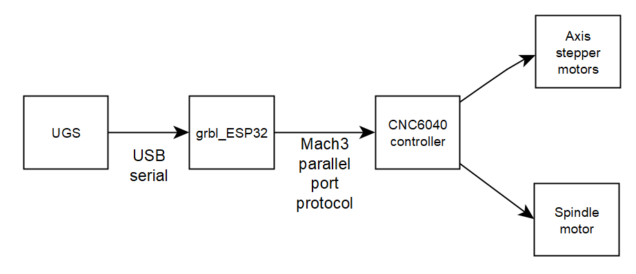
Above is the system block diagram. The grbl_ESP32 gcode interpeter processes a gcode S (speed) command, converting it to a variable duty cycle PWM waveform on parallel port pin 1. Continue reading CNC6040 router project – spindle speed linearisation

Noise Figure Y factor method calculator updated

Recent updates to Noise Figure Y factor method calculator expose the temperature of each of the attenuators in each scenario and so allow more flexibility in application to real world problems.

The screenshot above demonstrates its use where the DUT and Att12 are cryogenically cooled.

For most applications, the default value of 290K is appropriate, so though the form has a few more fields, there isn’t more data entry for most usage.

The calcs have not changed, just replacement of a global Tatt with T for each instance. The input form and output form have been reformatted to suit.


Noise Figure – Equivalent Noise Bandwidth

Harald Friis (Friis 1944) gave guidance on measuring the noise figure of receivers, and explains the concept of Effective Bandwidth.

Effective Bandwidth

The contribution to the available output noise by the Johnson-noise sources in the signal generator is readily calculated for and ideal or square-top band-pass characteristic and it is GKTB where B is the bandwidth in cycles per second. In practice, however, the band is not flat; ie, the gain over the band is not constant but varies with frequency. In this case the total contribution is ∫GfKTdf where Gf is the gain at frequency f. The effective bandwidth B of the network is defined as the bandwidth of an ideal band-pass network with gain G that gives this contribution to the noise output.

Continue reading Noise Figure – Equivalent Noise Bandwidth

nanovna-saver – a first look

The NanoVNA is a new low cost community developed VNA with assembled units coming out of China for <$50.

I have long held the view that these things are most useful when accompanied by a capable PC client that performs flexible text book presentations of data.

Considering buying one, my first step was to perform a desk evaluation of a popular PC client, which seems to be nanovna-saver.

Before downloading it, I examined the first screenshot on the github page.

It gives evidence that the author does not follow industry standard convention for transmission line terms and theory.

In the results shown above (s11) impedance is 39.105+j39.292Ω and some transformations of that value. Continue reading nanovna-saver – a first look

Is it 290K or 293K?

A reader of my articles commented on them and some of my calculators regarding the use of 290K as the reference temperature (T0) for Noise Figures.

(Friis 1944) suggested that temperature as reference temperature and it has been widely used since. One may also see 293K (eg in certain ITU-R recommendations), but in my experience, 290K is most commonly used and is for instance the basis for calibration of Keysight noise sources in Excess Noise Ratio (ENR).

The assumption in measurement of Noise Figure or of sensitivity is that the ‘cold’ source has a known source resistance with Johnson noise equivalent to 290K (16.85° C). That noise producing resistance is commonly achieved using a large attenuator at the generator output.

References / links

  • Friis, HT. Noise figures of radio receivers. Proceedings of the IRE, Jul 1944 p420.
  • Keysight. Jul 2018. Keysight 346A/B/C noise source operating and service manual.