NEC model of figure 8 transmitting loop

Variants of loops have been designed and promoted as having certain advantages, and one of those is the so-called figure 8 loop.

This article describes an NEC-4.2 model at 14MHz of an antenna similar to a commercial example.

The graphic shows the geometry. In this case the source is at the bottom of the lower loop, and the blue square is the tuning capacitor. The loop conductor is 22mm copper tube, the loop diameters are 1m, and the capacitor connection is 100mm wide. Commonly these are fed by a low loss auxiliary loop at the bottom of the lower loop, but the direct feed is quite fine for modelling the loop performance. Continue reading NEC model of figure 8 transmitting loop

nanoVNA-H – a summary of the experience so far

The NanoVNA is a new low cost community developed VNA with assembled units coming out of China for <$50.

I purchased what appears to be a ‘genuine’ nanoVNA-H and it has firmware NanoVNA-H_20191018.dfu installed. During checkout of the delivered device, an issue became evident, an issue worth describing in its own article.

Nevertheless, one online expert assured me it is a fake because genuine ones use green solder mask. Continue reading nanoVNA-H – a summary of the experience so far

The system wide conjugate match stuff crashes out again

Walt Maxwell (W2DU) made much of conjugate matching in antenna systems, he wrote of his volume in the preface to (Maxwell 2001 24.5):

It explains in great detail how the antenna tuner at the input terminals of the feed line provides a conjugate match at the antenna terminals, and tunes a non-resonant antenna to resonance while also providing an impedance match for the output of the transceiver.

Walt Maxwell made much of conjugate matching, and wrote often of it as though at some optimal adjustment of an ATU there was a system wide state of conjugate match conferred, that at each and every point in an antenna system the impedance looking towards the source was the conjugate of the impedance looking towards the load.

This was recently cited in a discussion about techniques to measure high impedances with a VNA:

WHEN the L and C’s of the tuner are set to produce a high performance return loss as measured by the vna, then in essence, if the tuner were terminated (where the vna was positioned) with 50 ohms and we were to look into the TUNER where the antenna was connected, we would see the ANTENNA Z CONJUGATE. Wow, that’s a mouth full. The best was to see this is to do an example problem and a simulator like LT Spice is a nice tool to learn. Or there are other SMITH GRAPHIC programs that are quite helpful to assist in this process. Standby and I will see what I can assemble.

The example subsequently described set about demonstrating the effect. The example characterised a certain antenna as having an equivalent circuit of 500Ω resistance in series with 4.19µH of inductance and 120pF of capacitance (@ 7.1MHz, Z=500-j0.119, not quite resonant, but very close). A lossless L network (where do you get them?) was then found that gave a near perfect match to 50+j0Ω. The proposition is that if you now look into the L network from the load end, that you see the complex conjugate of the antenna, Z=500+j0.119.

I asked where do you get a lossless L network? Only in the imagination, they are not a thing of the real world. Continue reading The system wide conjugate match stuff crashes out again

nanoVNA-H – sweep of a coax line section with OC termination

This article discusses the use of the (modified) nanoVNA-H raw accuracy and the implications for calibrated measurements.

Introduction

VNAs achieve much of their accuracy by applying a set of error corrections to a measurement data set.

The error corrections are obtained by making ‘raw’ measurements of a set of known parts, most commonly a short circuit, open circuit and load resistor (the OSL parts). The correction data may assume each of these parts is ideal, or it may provide for inclusion of a more sophisticated model of their imperfection. This process is known as calibration of the instrument and test fixture. nanovna-Q appears to have some fixed departure compensation to suit the SMA cal parts, less suited to other test fixtures.

So, when you make a measurement at some frequency, the correction data for THAT frequency is retrieved and used to correct the measurement.

What if there is not correction data for THAT frequency? There are two approaches:

  • a calibration run is required for exactly the same frequency range and steps (linear, logarithmic, size) as the intended measurement; and
  • existing calibration data is interpolated to the frequency of interest.

The interpolation method is convenient, but adds uncertainty (error) to the measurement. Some commercial VNAs will NOT interpolate.

The nanoVNA will interpolate, and with interpolation comes increased uncertainty.

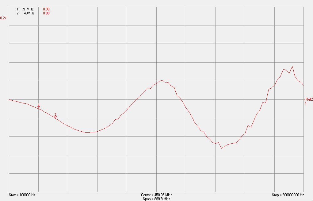
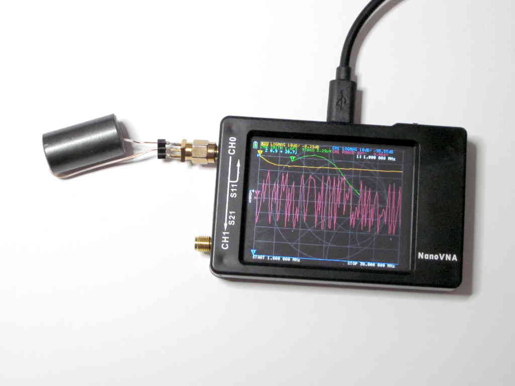
An uncorrected sweep of a reasonably known DUT is revealing of the instrument inherent error.

The DUT is a 12m length of LMR400.

Expected behavior

Let’s first estimate how it should behave.

The VNA contains a directional coupler nominally designed / calibrated for Zo=50+j0Ω, and in use, VNAs are invariably used to display measurements in terms of some purely real impedance, commonly 50Ω.

Though the DUT characteristic impedance (Zo) is nominally 50Ω, it is not EXACTLY 50+j0Ω and so there are departures in the displayed values wrt 50Ω from what might happen in terms of the actual Zo.

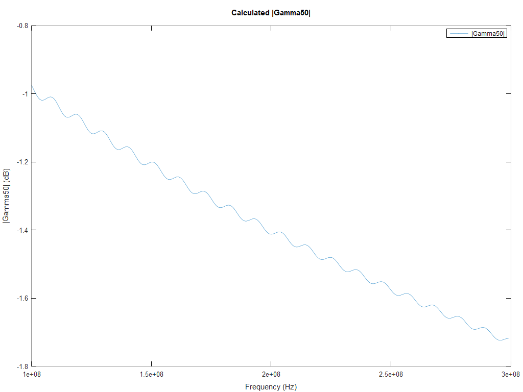
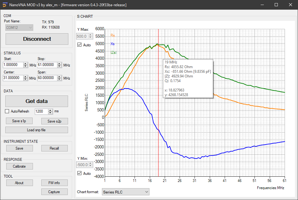
We can calculate the magnitude of Gamma for our 12m OC section of LMR400 over a range of frequencies.

|Gamma| vs frequency is a smooth curve as a result of line attenuation increasing with frequency. As a result in the small departure in Zo, |Gamma| wrt 50Ω has a superimposed small decaying oscillation. Continue reading nanoVNA-H – sweep of a coax line section with OC termination

nanoVNA-H – T-Check test

Rhode & Schwarz describe a test for accuracy of a VNA at T-Check Accuracy Test for Vector Network Analyzers utilizing a Tee-junction.

A nanoVNA-H PCB v3.3 (modified to fix decoupling problem on mixers) was calibrated from 0.1-900MHz using the supplied parts.

A T piece with extra 50Ω termination was inserted between the supplied original cables and s11 and s21 captured. The assembly was turned around and measured again to capture s22 and s12 (though recorded as s11 and s21). The two files were merged to obtain a full two port bothways .s2p file.

The T-Check value was calculated and is plotted here in VNWA.

Above, the T-Check results are not stunning at all, the ideal result is 1.0 at all frequencies. Rhode and Schwarz recommend that more than 15% error is unacceptable… of course that is in a commercial grade VNA.

nanoVNA-H – measure ferrite transformer

This article demonstrates the use of the (modified) nanoVNA-H to measure Loss (Transmission Loss) and Insertion Loss of a small ferrite 64:1 RF transformer, and the Insertion VSWR and Return Loss. The transformer was designed for a receive application at 9MHz.

Firstly let’s define the meaning of the terms: Continue reading nanoVNA-H – measure ferrite transformer

nanoVNA-H – measure ferrite core permeability

This article demonstrates the use of the (modified) nanoVNA-H to capture data from which the complex relative permeability of an unknown ferrite core is calculated and plotted

Above, a single turn of wire through the sleeve allows measurement by the nanovna. The nanoVNA fundamentally captures s11 parameters which we need to convert to relative permeability. Continue reading nanoVNA-H – measure ferrite core permeability

nanoVNA-H – measure equivalent core loss resistance

A very common design of a n:1 transformer for EFHW antennas uses a 2t primary on and FT240-43 (or even smaller) ferrite core.

In a process of designing a transformer, we often start with an approximate low frequency equivalent circuit. “Low frequency” is a relative term, it means at frequencies where each winding current phase is uniform, and the effects of distributed capacitance are insignificant.

Above is a commonly used low frequency equivalent of a transformer. Z1 and Z2 represent leakage impedances (ie the effect of magnetic flux leakage) and winding conductor loss. Zm is the magnetising impedance and represents the self inductance of the primary winding and core losses (hysteresis and eddy current losses). Continue reading nanoVNA-H – measure equivalent core loss resistance

nanoVNA-H – a ferrite cored test inductor impedance measurement – s21 series vs s11 reflection

One often sees experts online insisting that s11 reflection impedance measurements of common mode chokes is inaccurate, and the ONLY way is s21 series measurement.

This one is built upside down so the connections are visible.

In this experiment using the SDR-KITS VNWA testboard (above), a series of measurements are made of an inductor, and the test setup.

The nanoVNA-H (modified) was calibrated using the test board and its associated OSL components. The test board is used without any additional attenuators, it is directly connected to the nanoVNA-H using 200mm RG174 fly leads.

s11 reflection measurement

Above is the s11 reflection measurement. It is quick, and most tools directly display R and X vs frequency (though some of the new age tools display X as pF or µH equivalents). This is nanoVNA MOD v3 (a derivative of nanovnasharp).

Ok, so we have 4856-j852Ω. Continue reading nanoVNA-H – a ferrite cored test inductor impedance measurement – s21 series vs s11 reflection