Discussion of WA7ARK’s contribution to a QRZ thread on an End Fed Dipole

In another long running discussion on QRZ about End Fed Antennas, WA7ARK offered a contribution:

(1) Back in post #30 I showed that with a halfwave wire fed close to its end works just like the same wire fed in the center; the only difference being the feed point impedance. I let EzNec figure this out; I didn’t have to explain it with any mysterious “displacement” currents. Shown as (1) in the attached.

Since, in the model, the source is a constant current source, that forces the current on either side of the source to be equal, and the radiation pattern predicted by EzNec reflects that, because the patterns for the end-fed and center-fed match… (go back and look at post #30)

His post #30 is of a 67′ dipole at 66′ above poor ground @ 7.18MHz, fed at one end.

Above is the current distribution of my approximate re-creation of his model in NEC-4.2. It reconciles with his published graphs. Continue reading Discussion of WA7ARK’s contribution to a QRZ thread on an End Fed Dipole

woolly thinking on the nature of feed line common mode current

An online expert somewhat exasperated that the audience hasn’t absorbed his wisdom elaborated in apparently many previous posts said:

We’ve been round and round on this discussion but in a current mode balun aka a common mode choke the losses due to the windings and core are common mode not differential mode losses. You DO NOT dissipate your transmitted and received signals, which are carried as differential mode signals, as choke losses.

I know you’ve been reminded of this many times and don’t expect you to accept it now but that’s how common mode chokes work.

Now there is a sense in ham radio forums that repetition transforms assertions to fact, but setting that aside, let’s look at the assertion from an energy conservation point of view. Continue reading woolly thinking on the nature of feed line common mode current

Hobbyking 2500mAh 18650 LiIon cells (9210000181-0) initial capacity test

This article is documentation of a capacity test of 5 x Hobbyking 2500mAh 18650 LiIon cells (9210000181-0).

The cells were purchased on 26/02/2018 (~$7 + shipping) and received at about 30% charge. They were each charged in a XTAR VC2 Plus charger at 0.5A until charged.

The cells are 65mm long, and do not claim to contain protection modules which are prudent in some applications.

Each cell was then discharged at 1A (0.4C) to 2.8V, the discharge was captured.
Continue reading Hobbyking 2500mAh 18650 LiIon cells (9210000181-0) initial capacity test

Aluminium ground system suitability for ham radio station

I have been asked a few times about my article Implementation of G5RV inverted V using high strength aluminium MIG wire, and conversations ran to the suitability of the wire to a radial system on Marconi type antennas.

Firstly, a progress report on the antenna, no news to report and that is good news, there have been no issues so far. Inspection of connections without disassembly has not shown signs of corrosion or fatigue. Continue reading Aluminium ground system suitability for ham radio station

Baluns – wire size insanity

An online expert recently expounded on detailed design of a balun, this is an excerpt about wire sizing.

The wire gauge used limits the current handling capacity of the wire, run too thin a wire and it will heat up. Run much too thin of a wire for the power in use and it will fuse open. Current carrying capacity of wire is typically rated for either power transmission applications or chassis wiring applications. The latter, and higher, current capacity for a wire is relevant to designing a balun. How much current your 50 watt signal generates depends on the impedance its looking into. If you’re talking about a 50 ohm system, with a perfect match you’ll deliver one amp through your balun wires when driving 50 watts into it. Allowing for say a 4:1 SWR the worst case current(@12.5 ohms) is 2 amps. If you’re using this as a tuner balun, perhaps to drive a multi-band doublet then the impedance can vary widely so over sizing the wires is easy insurance. Here’s a table of wire current carrying capability: https://www.powerstream.com/Wire_Size.htm

For convenience, the relevant part of the table linked above is quoted for discussion.

So, the poster recommends wire with chassis wiring rating of 2A for 50W with reserve capacity for worst case VSWR=4. Continue reading Baluns – wire size insanity

ARRL guidance on design of ferrite cored inductors

The ARRL handbook for radio communications (Ward 2011) gives guidance on designing with ferrite cored inductors:

Ferrite cores are often unpainted, unlike powdered-iron toroids. Ferrite toroids and rods often have sharp edges, while powdered-iron toroids usually have rounded edges.
Because of their higher permeabilities, the formulas for calculating inductance and turns require slight modification. Manufacturers list ferrite AL values in mH per 1000 turnssquared. Thus, to calculate inductance, the formula is

L=ALxN2/1000000

where:

L = the inductance in mH
AL = the inductance index in mH per 1000 turns-squared, and
N = the number of turns.

Example: What is the inductance of a 60-turn inductor on a core with an AL of 523? (See the chapter Component Data and References for more detailed data on the range of available cores.)

L=ALxN2/1000000=523×602/1000000=1.88e6/1e6=1.88mH

Lets follow the example through. Continue reading ARRL guidance on design of ferrite cored inductors

Antenna half power bandwidth and Q, concept and experimental validation

Many antennas can be represented near their series resonance as a series RLC circuit, and in many cases R changes very slowly with frequency compared to X. This provides a convenient and good approximation for the behavior of the antenna impedance in terms of a simple linear circuit.

Series resonant circuit

The response of a simple series resonant RLC circuit is well established, when driven by a constant voltage source the current is maximum where Xl=Xc (known as resonance) and falls away above and below that frequency. In fact the normalised shape of that response was known as the Universal Resonance Curve and used widely before more modern computational tools made it redundant.

Above is a chart of the Universal Resonance Curve from (Terman 1955). The chart refers to “cycles”, the unit for frequency before Hertz was adopted, and yes, these fundamental concepts are very old. Continue reading Antenna half power bandwidth and Q, concept and experimental validation

IMD associated with colorbond sheet steel cladding

A recent experiment exposed significant IMD of a 7MHz locally radiated signal.

The source used for these tests is a battery powered low power transmitter  driving a 0.6m square loop. Radiated power is very low (of the order of -60dBm EIRP), and received signal on the station receiver is less than -73dBm.

Loop near steel shed #1

The loop was leaned against the colorbond sheet steel wall of shed #1. Shed #1 is about 40m from the receiving antenna, and is connected to the power mains. The building has colorbond sheet steel screwed to a steel frame. Colorbond is painted Zinc/Aluminium coated steel.

For this test, the submain was turned off at the main switchboard, so there is not equipment in the shed powered up, but the supply neutral is still connected and bonded to the shed steel work and shed PES ground electrode.

Above, the spectral response of receiver output, there are a number of side products at 100Hz intervals, presumably some form of IMD. At higher radiated power, products at odd 50Hz intervals become visible, though at much lower level than the 100Hz products. Continue reading IMD associated with colorbond sheet steel cladding

Baselining an antenna system with an analyser

I often receive emails from folk trying to validate continued performance of an installed antenna system using their analyser.

With foresight they have swept the antenna system from the tx end and saved the data to serve as a baseline.

The following are example sweeps from one of my own antennas, a Diamond X50N with 10m of LDF4-50A feed line.

Now I have plotted Return Loss rather than VSWR for several reasons:

  • Return Loss is more sensitive to the problems that we might want to identify;
  • Rigexpert in this case decided that the Antscope user could not be interested in plotting VSWR>5 (Return Loss<3.5dB).

Now a hazard in working with Return Loss is that many authors of articles and software don’t use the industry standard meaning.

Return Loss

Lets just remind ourselves of the meaning of the term Return Loss. (IEEE 1988) defines Return Loss as:

(1) (data transmission) (A) At a discontinuity in a transmission system the difference between the power incident upon the discontinuity. (B) The ratio in decibels of the power incident upon the discontinuity to the power reflected from the discontinuity. Note: This ratio is also the square of the reciprocal to the magnitude of the reflection coefficient. (C) More broadly, the return loss is a measure of the dissimilarity between two impedances, being equal to the number of decibels that corresponds to the scalar value of the reciprocal of the reflection coefficient, and hence being expressed by the following formula:

20*log10|(Z1+Z2)/(Z1-Z2)| decibel

where Z1 and Z2 = the two impedances.

(2) (or gain) (waveguide). The ratio of incident to reflected power at a reference plane of a network.

Return Loss expressed in dB will ALWAYS be a positive number in passive networks.

The relationship between ReturnLoss in dB and VSWR is given by the equations:

  • ReturnLoss=-20*log((VSWR-1)/(VSWR+1))
  • VSWR=(1+10^(-ReturnLoss/20))/(1-10^(-ReturnLoss/20))

Diamond X50N on 2m

So now that we are on the same page about Return Loss, lets look at my 2m plot.

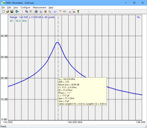
The X50N does not have VSWR or Return Loss specs, but we might expect that at the antenna itself, VSWR<1.5 which implies Return Loss>25dB. Measuring into feed line, you can add twice the matched line loss to the Return Loss target (see why Return Loss is a better measure).
Continue reading Baselining an antenna system with an analyser

Thompson’s coax common mode explanation

A recent online discussion on common mode feed line current was directed to Thompson’s article with the recommendation that is ALL basically needed to discuss the common mode current.

Above is Thompson’s diagram of currents in a feed coax, and it contains two significant errors that could / would lead to formation of the wrong concepts in a learner’s mind. Continue reading Thompson’s coax common mode explanation