The devil is in the detail – real world transmission lines and loss under standing waves

We are traditionally taught transmission line theory starting with the concept of complex propagation constant γ, and that loss in a section of line is \(Loss=20log_{10}( l |\gamma|) dB\) where l is length. That is the ‘one way’ loss in a travelling wave, also the the matched line loss (MLL) (as there is no reflected wave).

There are some popular formulas and charts that purport to properly estimate the loss under standing waves or mismatch conditions, usually in the form of a function of VSWR and MLL, more on this later.

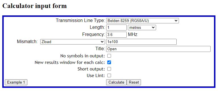
Let’s explore theoretical calculations of loss for a very short section of common RG58 at 3.6MHz with two different load scenarios.

The scenarios are:

  • Zload=5+j0Ω (VSWR50=10); and
  • Zload=500+j0Ω (VSWR50=10).

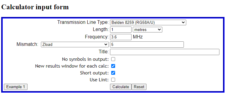
Above is the RF Transmission Line Loss Calculator (TLLC) input form. A similar case was run for Zload=500Ω. Continue reading The devil is in the detail – real world transmission lines and loss under standing waves

The devil is in the detail – real world transmission lines and ReturnLoss

We are traditionally taught transmission line theory starting with the concept of complex propagation constant γ and then dealing with them as lossless lines (means Zo is purely real) or low loss distortionless lines (means Zo is purely real).

Let’s explore theoretical calculations of ReturnLoss for a very short section of common RG58 at 3.6MHz.

By definition, \(ReturnLoss=\frac{ForwardPower}{ReflectedPower}\) and it may be expressed as \(ReturnLoss=10log_{10}\frac{ForwardPower}{ReflectedPower} dB\).

The scenarios are:

  • open circuit termination; and
  • short circuit termination.

Above is the RF Transmission Line Loss Calculator (TLLC) input form. Note that it will not accept Zload of zero or infinity, instead a very small value (1e-100) or very large value (1e100) is used. Continue reading The devil is in the detail – real world transmission lines and ReturnLoss

Measurement of recent ‘FT240-43’ core parameters

This article reports measurement of two ‘FT240-43’ cores (actually Fair-rite 5943003801 ‘inductive’ toroids, ie not suppression product) purchased together around 2019, so quite likely from the same manufacturing batch. IIRC, the country of origin was given as China, it is so for product ordered today from element14. The measurements are of 1t on the core, with very short connections to a nanoVNA OSL calibrated from 1-50MHz.

Above, the measurement fixture is simply a short piece of 0.5mm solid copper wire (from data cable) zip tied to the external thread of the SMA jack, and the other end wrapped around the core and just long enough to insert into the inner female pin of the SMA jack. Continue reading Measurement of recent ‘FT240-43’ core parameters

nanoVNA – RG6/U with CCS centre conductor MLL measurement

In my recent article RG6/U with CCS centre conductor – shielded twin study I made the point that it is naive to rely upon most line loss calculators for estimating the loss of this cable type partly because of their inability to model the loss at low HF and partly because of the confidence one might have in commonly available product. In that article I relied upon measured data for a test line section.

I have been asked if the nanoVNA could be bought to bear on the problem of measuring actual matched line loss (MLL). This article describes one method.

The nanoVNA has been OSL calibrated from 1-299MHz, and a 35m section of good RG6 quad shield CCS cable connected to Port 1 (Ch0 in nanoVNA speak).

A sweep was made from 1-30MHz with the far end open and shorted and the sweeps saved as .s1p files.

Above is a screenshot of one of the sweeps. Continue reading nanoVNA – RG6/U with CCS centre conductor MLL measurement

RG6/U with CCS centre conductor – shielded twin study

Some online experts advise the use of synthesised shielded twin instead of ordinary two wire line for HF antennas claiming it is vastly superior.

Now it could be vastly superior for several reasons in all, but let’s focus on just one important parameter, loss under mismatch conditions.

The scenario then is the very popular 132′ multi band dipole:

  • the famous 40m (132′) centre fed dipole;
  • 20m of feed line being parallel RG6/U CCS quad shield with shields bonded at both ends;
  • 7MHz where we will assume dipole feed point impedance is ~4000+j0Ω.

We will consider the system balanced and only deal with differential currents.

Now rather than depend on loss calculators, most of which don’t reconcile with measurement of CCS RG6/U, I will used measured loss. RG6/U with CCS centre conductor at HF gives a chart of measured loss of a sample of commercial grade CCS quad shield coax.

Above is a comparison of matched line loss (MLL) based on measurement of a length of RG6/U Quad Shield CCS cable and prediction from Simsmith of Belden 8215 (also CCS). The ripple is due to measurement system error, measurements were made quite some years ago with a AIMuhf. Continue reading RG6/U with CCS centre conductor – shielded twin study

nanoVNA – measuring cable velocity factor – demonstration – open wire line

The article nanoVNA – measuring cable velocity factor – demonstration demonstrated measurement of velocity factor of a section of coaxial transmission line. This article demonstrates the technique on a section of two wire copper line.

A significant difference in the two wire line is that we want the line to operate in balanced mode during the test, that there is insignificant common mode current. To that end, a balun will be used on the nanoVNA.

Above, the balun is a home made 1:4 balun that was at hand (the ratio is not too important as the fixture is calibrated at the balun secondary terminals). This balun is wound like a voltage balun, but the secondary is isolated from the input in that it does not have a ‘grounded’ centre tap. There is of course some distributed coupling, but the common mode impedance is very high at the frequencies being used for the test. Continue reading nanoVNA – measuring cable velocity factor – demonstration – open wire line

nanoVNA – experts on improvised fixtures

A newbie wanting to measure a CB (27MHz) antenna with a UHF plug when his nanoVNA has an SMA connector sought advice of the collected experts on groups.io.

One expert advised that 100mm wire clip leads would work just fine. Another expert expanded on that with When lengths approach 1/20 of a wavelength in free space, you should consider and use more rigorous connections.

At Antenna analyser – what if the device under test does not have a coax plug on it? I discussed using clip leads and estimated for those shown that they behaved like a transmission line segment with Zo=200Ω and vf=0.8. Continue reading nanoVNA – experts on improvised fixtures

Simsmith bimetal line type – revision #1

This article is a revision of an article Simsmith bimetal line type for Simsmith v17.2 and revisions to my own model for current distribution in a conductor.

This article discusses various measurements and models of Wireman 551 windowed ladder line, including adapting Simsmith’s bimetal line type to bear on the problem.

Measurements

A starting point for characterising the matched line loss (MLL) of the very popular Wireman 551 (W551) windowed ladder line is the extrapolation of measurements by (Stewart 1999) to 1.8MHz. Since the measurements were made at and above 50MHz where the W551 has copper like performance, this is likely to underestimate actual MLL and such wide extrapolation introduces its own uncertainty. Nevertheless, the datapoint is MLL=0.00227dB/m.

This is a revision of an article written in Feb 2020, capturing revision of Simsmith to v17.2 and revision of my own current distribution model.

Dan Maquire recently posted a chart summarising measurements of these lines.

For the purposes of this article, let’s tabulate the MLL at 1.8MHz in dB/m. Continue reading Simsmith bimetal line type – revision #1

A model of current distribution in copper clad steel conductors at RF – capturing conductor curvature

A model of current distribution in copper clad steel conductors at RF laid out a model for current distribution, though ignoring curvature of the conductor in calculating current density vs depth.

A model for current distribution in a conductor is that for a homogenous conducting half space with surface current parallel to the interface. Current density at depth d is given by the expression \(J_r=J_R\frac{J_0(kr)}{J_0(kR)}\) where δ is the skin depth \(δ=(ω \cdot µ \cdot σ)^{0.5}\) and \(k=\frac{1-\jmath}{\delta}\), σ is the conductivity). This takes into account curvature of the conductor surface, albeit with slower compute time.

Let’s compare the two algorithms on a test case at 1.8MHz being copper cladding of 67µm copper over a steel core for an overall diameter of 1.024mm (#18).

Above is a stacked image, the simpler algorithm is the feint plot.

There is a quite small difference in this case. When the expected loss of 400Ω line using the conductor is calculated, the result with the simpler algorithm is 1.3% less than the later one using the Bessel distribution.

Distance to fault in submarine telegraph cables ca 1871 – the leap expanded

Distance to fault in submarine telegraph cables ca 1871 gave a mathematical explanation of the location of fault…

Now it is in terms of the three known values u,v,w and unknown x.

\(w(v-2x+u)=(v-2x+u)x+(v-x)(u-x)\\\)

\(x^2-2wx+vw+uw-uv=0\) from which you can find the roots.

\(x=w – \sqrt{(w-v)(w-u)}\\\)

I have been asked to expand the last ‘leap’.

So we have \(x^2-2wx+vw+uw-uv=0\) which is a quadratic, a polynomial of order 2.

The solution or roots of a quadratic \(ax^2+bx+c=0\) are given by \(x=\frac{-b \pm \sqrt{b^2-4ac}}{2a}\).

So, for our quadratic \(a=1, b=-2w,c=vw+uw-uv\), so \(x=\frac{2w \pm \sqrt{(2w)^2-4(vw+uw-uv)}}{2}\).

Dividing the top and bottom by 2 we get \(x=w \pm \sqrt{w^2-(vw+uw-uv)}\) which can be rewritten as \(x=w \pm \sqrt{(w-v)(w-u)}\).

We want the lesser square root \(x_-=w-\sqrt{(w-v)(w-u)}\) because x must be less than w, a constraint of the physical problem.

So when measurements gave \(v=1040 \Omega\) and \(w=970 \Omega\) we can calculate that the distance to fault is the lesser root, 210.3km from Newbiggen-by-the-sea. (The greater root would imply a -ve value for x or y which is not physically possible.)