Calculate Loss from s11 and s21 – convenient online calculator

I often need to calculate loss from marker values on a VNA screen, or extracted from a saved .s2p file.

Firstly, loss means PowerIn/PowerOut, and can be expressed in dB as 10log(PowerIn/PowerOut). For a passive network, loss is always greater than unity or +ve in dB.

\(loss=\frac{PowerIn}{PowerOut}\\\)

Some might also refer to this as Transmission Loss to avoid doubt, but it is the fundamental meaning of loss which might be further qualified.

So, lets find the two quantities in the right hand side using ‘powerwaves’ as used in S parameter measurement.

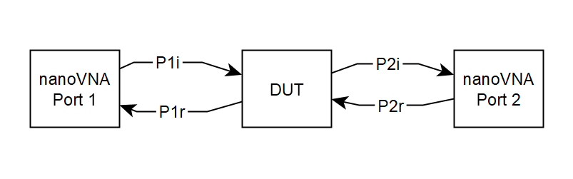
s11 and s21 are complex quantities, both relative to port 1 forward power, so we can use them to calculate relative PowerIn and relative PowerOut, and from that PowerIn/PowerOut.

PowerIn

PowerIn is port 1 forward power less the reflected power at port 1, \(PowerIn=P_{fwd} \cdot (1-|s11|^2)\).

PowerOut

PowerOut is port 2 forward power times less the reflected power at the load (which we take to be zero as under this test it is a good 50Ω termination), \(PowerOut=P_{fwd} \cdot |s21|^2 \).

Loss

So, we can calculate \(loss=\frac{PowerIn}{PowerOut}=\frac{\frac{PowerIn}{P_{fwd}}}{ \frac{PowerOut}{P_{fwd}}}=\frac{1-|s11|^2}{|s21|^2}\)

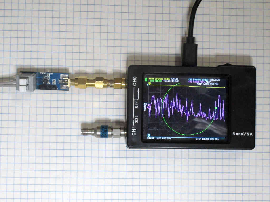
Noelec makes a small transformer, the Balun One Nine, pictured above and they offer a set of |s11| and |s12| curves in a back to back test. (Note: back to back tests are not a very reliable test.) Continue reading Calculate Loss from s11 and s21 – convenient online calculator

Measure transmission line Zo – nanoVNA – PVC speaker twin

There are many ways to get a good estimate of the characteristic impedance Zo of a transmission line.

One method is to measure the input impedances of a section of line with both a short circuit and open circuit termination. From Zsc and Zoc we can calculate the Zo, and the complex propagation constant \(\gamma=\alpha + \jmath \beta\), and from that, MLL.

Calculation of Zo is quite straightforward.

The solution for γ involves the log of a complex number \(r \angle \theta\) which is one of the many possible values \(ln(r) + j \left(\theta + 2 \pi k \right)\) for +ve integer k. Conveniently, the real part α is simply \(ln(r) \). The real part of γ is the attenuation in Np/m which can be scaled to dB/m, and the imaginary part is the phase velocity in c/m. The challenge is finding k.

Measurement with nanoVNA

So, let’s measure a sample of 14×0.14, 0.22mm^2, 0.5mm dia PVC insulated small speaker twin.

Above is the nanoVNA setup for measurement. Continue reading Measure transmission line Zo – nanoVNA – PVC speaker twin

Measure transmission line Zo – nanoVNA – CCS RG6

There are many ways to get a good estimate of the characteristic impedance Zo of a transmission line.

One method is to measure the input impedances of a section of line with both a short circuit and open circuit termination. From Zsc and Zoc we can calculate the Zo, and the complex propagation constant \(\gamma=\alpha + \jmath \beta\), and from that, MLL.

Calculation of Zo is quite straightforward.

The solution for γ involves the log of a complex number \(r \angle \theta\) which is one of the many possible values \(ln(r) + j \left(\theta + 2 \pi k \right)\) for +ve integer k. Conveniently, the real part α is simply \(ln(r) \). The real part of γ is the attenuation in Np/m which can be scaled to dB/m, and the imaginary part is the phase velocity in c/m. The challenge is finding k.

Let’s take an example from recent measurements of 35m of CCS RG6 coax, and extract the s11 values recorded in saved .s1p files @ 1.87MHz. The saved data in MA format, magnitude and angle (in degrees).

Calculate Zo and gamma is flexible and can accept the MA format data directly.

Above, the results. Zo is 74.73-j1.156Ω, and matched line loss MLL is 0.03281dB/m. This MLL is quite a deal higher than you might find in many line loss calculators, they often fail on CCS cables. Continue reading Measure transmission line Zo – nanoVNA – CCS RG6

nanoVNA – touch screen problems

My nanoVNA-H v3.3 is just over six months old. It has succumbed to most of the common hardware faults and some of the less common ones, but until now the touch screen has worked ok.

That has changed, the bezel bears on the touch screen and causes input when the case is held even very lightly by the edges… sufficiently so that it was unusable.

A perhaps temporary resolution was to place four 1mm thick M2 5mm OD nylon washers on the front part of the case before carefully placing the PCB assembly on top, then the case back and screws. This is a bit tedious if one of the washers moves, next time it is apart to fix hardware issues, I might put a dot of CA adhesive under each washer.

The case design is inadequate, it needed some features incorporated into the molding of the front to space the edges of the bezel off the PCB so that it maintained the requisite spacing even when held, even after the molding changes over time (perhaps normalisation of stresses from the molding process).

nanoVNA – measure Transmission Loss – example 5

This article is demonstration of measurement of Transmission Loss in a section of two wire transmission line embedded in a common mode choke. The scenario is based on an online article  MEASURING DM ATTENUATION of YOUR CMC USING THE NANOVNA AND NANOVNA SAVER.

The reference article publishes measured attenuation or loss being -1.45dB @ 28.4MHz. Of course, the -ve value hints that the author is lost in hamdom where all losses MUST be -ve dB..

The meaning of loss in a generic sense (ie without further qualification) is \(loss=\frac{Power_{in}}{Power_{out}}\) and can be expressed in dB as \(loss_{dB}=10 log_{10}(loss)\).

Some might interpret the result to imply that \((1-10^{\frac{-loss}{10}})*100=28 \%\) of input power is converted to heat in the choke.

The result given (and corrected) as 1.45dB was taken simply from the nanoVNA \(|s21|\) result, and so it is actually InsertionLoss, not simply Loss.

What is the difference? Continue reading nanoVNA – measure Transmission Loss – example 5

Disturbing the thing being measured – coax line

An issue that often arises in online discussions inability to reconcile the VSWR indicated by a transceiver (or possibly an inline VSWR meter) and an antenna analyser.

Is this Segal’s law at play?

There are several common contributors including:

  • faulty, dirty, or not properly mated connectors and cables;
  • VSWR meters that are not accurate at low power levels; and
  • influence of the common mode current path on VSWR.

Continue reading Disturbing the thing being measured – coax line

nanoVNA – measure Transmission Loss – example 4

This article is demonstration of measurement of Transmission Loss in a section of coaxial transmission line. The scenario is chosen to expose the experiment to some of the things that complicate such measurements.

The very popular nanoVNA-H will be used to make the measurements.

The scenario:

  • nanoVNA fully calibrated from 1.5-1.8MHz using a 200mm length coax lead on Port 2 (nanoVNA CH1);
  • 10m of RG58C/U; and
  • f=1.65MHz.

Above is a block diagram of the test configuration. nanoVNA measurements are wrt 50Ω, so \(P=\frac{V^2}{50}\) and \(V=\sqrt{50P}\). Continue reading nanoVNA – measure Transmission Loss – example 4

nanoVNA – measure Transmission Loss – example 3

This article is demonstration of measurement of Transmission Loss in a section of coaxial transmission line. The scenario is chosen to expose the experiment to some of the things that complicate such measurements.

The very popular nanoVNA-H will be used to make the measurements.

The scenario:

  • nanoVNA fully calibrated from 1-5MHz using a 200mm length coax lead on Port 2 (nanoVNA CH1);
  • 35m of CCS RG6/U (close to an electrical quarter wavelength);
  • 75-50Ω Minimum Loss Pad (5.72dB); and
  • f=1.65MHz (close to a quarter wavelength.

Above is a block diagram of the test configuration. nanoVNA measurements are wrt 50Ω, so \(P=\frac{V^2}{50}\) and \(V=\sqrt{50P}\). Continue reading nanoVNA – measure Transmission Loss – example 3

nanoVNA – measure Transmission Loss – example 2

This article is demonstration of measurement of Transmission Loss in a section of coaxial transmission line. The scenario is chosen to expose the experiment to some of the things that complicate such measurements.

The very popular nanoVNA-H will be used to make the measurements.

The scenario:

  • nanoVNA fully calibrated from 1-5MHz using a 200mm length coax lead on Port 2 (nanoVNA CH1);
  • 35m of CCS RG6/U (close to an electrical quarter wavelength);
  • three 50Ω terminations in shunt with VNA Port 2; and
  • f=1.65MHz (close to a quarter wavelength.

The transmission line load is four 50Ω loads in parallel, one of them being VNA Port 2. Only one quarter of the output power is captured by the VNA, so there is effectively a loss of 6.02dB in that configuration. It also delivers a 12.5+j0Ω load the the transmission lines, VSWR is about 6. Note this power division is based on the assumption that Zin of Port 2 is 50+j0Ω, and error in Zin flows into the result. A 10dB attenuator is fitted to Port 2 prior to calibration to improve accuracy of Zin.

Above is a block diagram of the test configuration. nanoVNA measurements are wrt 50Ω, so \(P=\frac{V^2}{50}\) and \(V=\sqrt{50P}\). Continue reading nanoVNA – measure Transmission Loss – example 2

nanoVNA – measure Transmission Loss – example 1

This article is demonstration of measurement of Transmission Loss in a section of coaxial transmission line. The scenario is chosen to expose the experiment to some of the things that complicate such measurements.

The very popular nanoVNA-H will be used to make the measurements.

The scenario:

  • nanoVNA fully calibrated from 1-5MHz using a 200mm length coax lead on Port 2 (nanoVNA CH1);
  • 35m of CCS RG6/U (close to an electrical quarter wavelength); and
  • f=1.65MHz (close to a quarter wavelength.

Above is a block diagram of the test configuration. nanoVNA measurements are wrt 50Ω, so \(P=\frac{V^2}{50}\) and \(V=\sqrt{50P}\). Continue reading nanoVNA – measure Transmission Loss – example 1