True balanced tuner

A recent long running thread on QRZ entitled “True balanced auto-tuner” was sure to tease out some pretty woolly thinking… the word “true” was enough to signal the outcome.

There are only three words in the title, we can dismiss “true” as a harbinger of woolly thinking, and though people will argue the toss on the appropriateness of the term “auto-tuner’, most people share an understanding of the meaning. “Balanced” is another problem altogether.

After thirty odd posts, there has been no definition or discussion of the term balanced, or its advantages or disadvantages.

One of the recommendations by several posters is the old is new again solution, the once popular link coupled tuner and the work of WZ5Q featured in one of those recommendations.

WZ5Q and WW8J

Topology

WZ5Q describes a tuner inspired by WW8J. WZ5Q extended the design and provides a writeup on optimising balance.

Above is WZ5Q’s partial circuit. In the article he describes and shows:

  • adjustment of the grounding point of the output tank; and
  • current meters which presumably attach to J2 and J3.

Key to analysis of the topology is that the centre of the output inductor is grounded. This results in the circuit tending towards equal but opposite phase voltages on the output terminals. Continue reading True balanced tuner

WSPR – data mining 40m 01/08/2017

I mentioned elsewhere that I dowloaded the WSPR archive for 1/08/2017, and particularly analysed 40m spots.

There were close to 1,000,000 spots for the day, about 340,000 on 40m, and about 20,000 individual transmissions reported during the day (40m).

Tx / Rx mix

Above is a pie chart of the mix of Tx Only, Rx ONLY and Tx/Rx stations. The largest group is Tx Only, 44% of stations do not contribute reception records. Nextly, 30% are Rx Only, and 27% Tx and Rx. Continue reading WSPR – data mining 40m 01/08/2017

WSPR checkout on 30m

On the back of A WSPR experiment for station evaluation I thought I would try a similar experiment on 30m in the quest for some meaningful results.

Given the lack of activity from credible stations on 40m, it seemed worth a checkout on 30m befor committing to the trial run, large download and data analysis.

So, I ran WSPR for a half hour just before 0000Z and observed the activity on WSPRnet map. I should note that my tx power was 0.1W and rx performance was impaired as there was a 20dB attenuator in line to achieve the tx power.

Above, the map after of the half hour of activity.

The encouraging this was that there were 12 stations active. Continue reading WSPR checkout on 30m

A WSPR experiment for station evaluation

An experiment was conducted on 40m using WSPR to compare my own station transmit performance with others relatively close by.

The experiment was conducted around sunset on 01/08/2017, data was collected for the period 0600Z to 0900Z, sunset was at 07:17Z.

The experiment was unannounced as previous experience has been that if the WSPR community becomes aware of activity that does not accord with individual’s opinion of acceptable, the activity can be disrupted.

Data for analysis was fetched by downloading the archive which contained nearly 1,000,000 records for the day, and about 340,000 of those were 40m spots.

Factors shaping experiment design

The following is a discussion of various factors that weighed into experiment design.

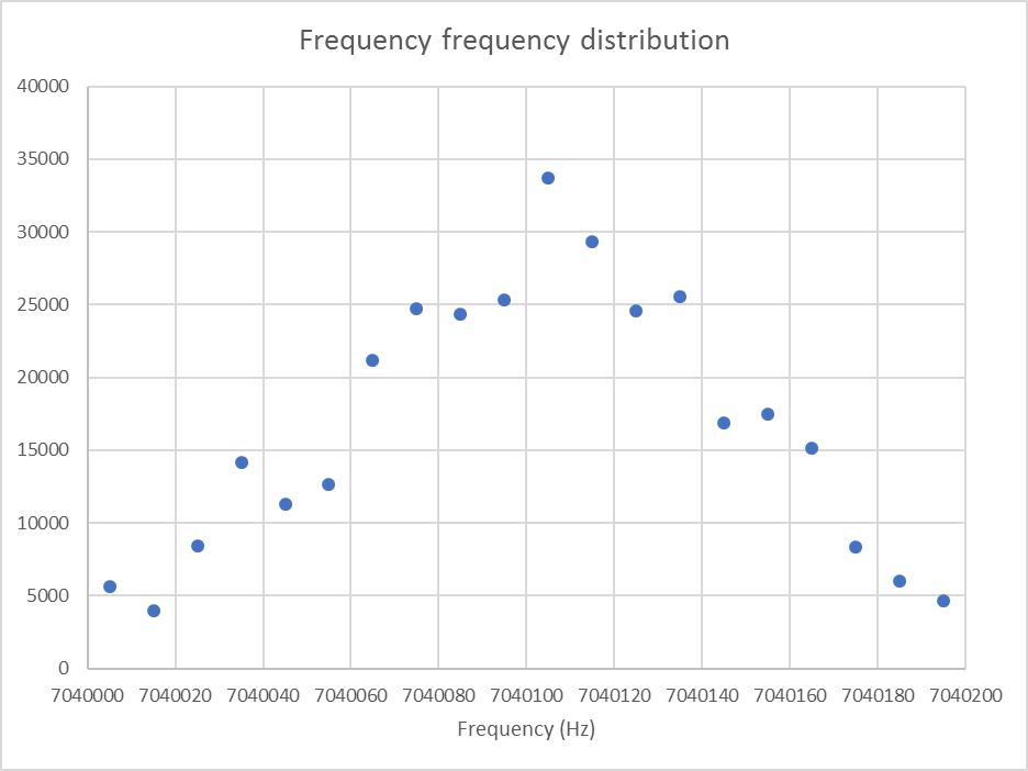
Transmitters tend to cluster around the centre of the 200Hz WSPR band.

Above is a frequency distribution of tx frequency, and it is evident that the risk of interference is reduced by choosing a frequency near the upper or lower limit of the band segment. There was some activity just outside the designated band segment which might indicate care and competence of operators.

One wonders if randomising the tx frequency might not reduce collisions and improve decode rates. Continue reading A WSPR experiment for station evaluation

Come-along from the past

I was working recently on an antenna and a visitor was intrigued by a device I was using.

Above, the device is for tensioning a wire span, commonly called a come-along though that term gets applied to all manner for appliances for broadly similar purpose. A significant difference is that this was designed for smooth hard drawn copper wires, and has smooth flat jaws (70x6mm) and does not put a kink in the wire (as do most wire grips for more general fencing and FSWR use). This one has had the strap replaced, it came with a 1.25″ canvas reinforced rubber transmission belt which became hard over time. Continue reading Come-along from the past

Implementation of G5RV inverted V using high strength aluminium MIG wire – impedance measurements

This article continues on from Implementation of G5RV inverted V using high strength aluminium MIG wire documenting impedance measurements and voltage calculations.

Impedance measurement

Impedance was measured with an AA-600 looking into 500mm of RG400 then the Guanella 1:1 balun, then 9m of fabricated transmission line as described in earlier articles in the series. The balun is located at the antenna entrance panel and the coax shield is grounded via that panel (ie the normal operating common mode current path exists).

Above is the impedance measurement plotted on a Smith chart. This is more useful and very meaningful as an interactive display in Antscope where are you move the cursor, the frequency and key data are displayed. Continue reading Implementation of G5RV inverted V using high strength aluminium MIG wire – impedance measurements

EME Calc v11.11 reconciliation issues

A correspondent wrote about trying to reconcile by G/T worksheet with EME Calc.

Many times I have tried to validate it and run into problems. At one time I reported them to the author, but they were never acknowledged, much less fixed.

The specific problem on this occasion relates to the receiver performance tab.

Above is a screenshot (with my annotations) where I have basically stripped the configuration down to a receiver attached to a noiseless antenna with lossless line. Continue reading EME Calc v11.11 reconciliation issues

Implementation of G5RV inverted V using high strength aluminium MIG wire

This article continues on from Workup of G5RV inverted V using high strength aluminium MIG wire and describes the implementation.

Above is a view of the steel mast with the Inverted V G5RV rigged from the top of the 11m mast using a halyard though a purchase on a small gibbet to offset the antenna and feed line from the mast. There are lateral guys at 7m height, and the left hand one is non-conductive synthetic fibre rope. Atop the mast is a 2m/70cm vertical. Continue reading Implementation of G5RV inverted V using high strength aluminium MIG wire

G3CWI’s ground wave tests Jul 2017 using WSPRlite

Richard (G3CWI) published an interesting blog article Comparison of groundwave performance of Small Transmitting Loop and Quarterwave GP summarising a recent WSPR test on 40m over 20km distance.

This article is a walk through of the expected WSPR receive S/N for the case of the 20mW tx on a quarter wave vertical.

100% efficient tx and rx antenna systems

Ground wave suffers attenuation due to two key components:

  1. dispersion of energy as the wave spreads out from the source; and
  2. absorption of energy in heating the soil.

Item (1) is simply inverse square law effect, and Norton provides us with several approximations for estimating (2) from Sommerfields work.

Calculate efficiency of vertically polarised antenna from far field strength uses Norton’s f5 approximation for ground wave attenuation.

Above is a calculation for a 100% efficient transmitter. (The trick to getting this is to leave the measured field strength field empty and the calculator will insert the value that gives 100% efficiency.)

So the next question is what ambient noise level might we expect in a rural setting on 40m. Continue reading G3CWI’s ground wave tests Jul 2017 using WSPRlite

Exploiting your antenna analyser #29

Resolving the sign of reactance – a method – Smith chart detail

Exploiting your antenna analyser #28 gave an example of use of one method to resolve the sign of reactance comparing measurements made with a slightly longer known transmission line.

One way to predict the input impedance to the longer line is using a Smith chart. This article presents a Smith chart prediction of the expected input impedance of a 8′ section of RG8 at 14.17Mhz (vf=0.66, length=0.175λ) for the cases of Zload being 60.3+j26.9Ω and  60.3-j26.9Ω.

60.3+j26.9Ω

The impedance is normalised to 50Ω and plotted on the Smith chart, point 1 above. A radial from the centre through point 1 is drawn to the edge of the chart. Another radial is drawn a distance towards the generator of 0.175λ and using a pair of dividers or ruler, point 2 is plotted on that radial at the same distance from the centre (same VSWR) as point 1.

These points are on a constant VSWR arc but the arc has not been draw because the two arcs would overlap and might be confusing to some readers.  Continue reading Exploiting your antenna analyser #29