Uncertainty of the noise sampling process
|
This article examines the uncertainty of the process of sampling noise for measurement, and a method for prediction of sampling uncertainty. The proposed solution has application generally to high resolution measurement of bandwidth limited noise. |
Characteristics of noise
Broadband noise is caused by a random process that generates a voltage that varies randomly over time.
The noise voltage is a normally distributed random variable.
Sampling is the process of converting a signal (for example, a function of continuous time or space) into a regular numeric sequence (a function of discrete time or space).
The noise voltage can be sampled, and the instantaneous power is proportional to the square of the sample value.
The average noise power can be estimated by averaging the instantaneous power at regular intervals over a period of time.
Pe=Σ(vi)2/n/R where Pe is the estimated noise power in a resistor, vi are the voltage samples, n is the number of samples and R is the load resistance.
It is important to remember that the measurement process is only an estimate of the true noise power, and that successive sample sets are likely to produce similar, but different estimates.
An explanation about the probability distribution of this sampling process can be obtained from classic statistics.
Statistically, the noise voltage samples are normally distributed, have a mean of zero, and a variance. The RMS voltage is equal to the square root of the variance.
If xi are independent normally distributed random variables with mean 0 and variance 1, then the random variable Q=Σxi2 is distributed according to the chi-square distribution. This is usually written as Q~χ2k.
The expression for Pe can be rewritten as Pe=v2/n/R*Σ(vi')2 where vi' is the normalised sample voltage such that its variance is 1, or Pe'=Σ(vi')2, and we can say that Pe'~χ2k (k=n-1).
Uncertainty
Since Pe'~χ2n, the critical points of the chi-square distribution can be used to find confidence limits for noise measurements based on an effective sample size.
 |
Remembering that the measurement process is only an estimate of the true noise power, and that successive sample sets are likely to produce similar, but different estimates. Fig 1 shows the probability that a measurement exceeds a given normalised power level for measurements based on 10,000 and 20,000 samples. The curves tell us that 90% of measurements based on 20,000 samples will indicate more than 0.987W (normalised power). Similarly, 10% of measurements based on 20,000 samples will indicate more than 1.013W, and so 90%-10% or 80% of measurements will be between 0.987W and 1.013W of the correct power. We can state that the sampling uncertainty is ±1.3% to a confidence level of 80%.
 |
Looking at Fig 2 which shows the probability that a measurement exceeds a given normalised power level for measurements based on 10,000 and 20,000 samples. The curves tell us that 90% of measurements based on 20,000 samples will indicate more than -0.06dB (normalised power). Similarly, 10% of measurements based on 20,000 samples will indicate more than 0.06dB, and so 90%-10% or 80% of measurements will be between -0.06dB and 0.06dB of the correct power. We can state that the sampling uncertainty is ±0.06dB to a confidence level of 80%.
 |
Fig 3 expands part of Fig 2. Looking at the curves, the 97.5% confidence limit for 20k samples is -0.086dB, and for 10k samples is -0.12dB. These results are summarised in Table 1.
| Sample set size | Sampling uncertainty (dB) |
| 10k | ±0.120 |
| 20k | ±0.086 |
Increasing sample set size reduces sampling uncertainty.
Effective sample set size
The Nyquist–Shannon sampling theorem states that exact reconstruction of a continuous-time baseband signal from its samples is possible if the signal is bandlimited and the sampling frequency is greater than twice the signal bandwidth.
This implies that a sample set with sampling frequency higher than twice the highest frequency, the Nyquist Rate, contains no more information than one with sampling frequency equal to the the Nyquist Rate.
Further, that translation of a limited bandwidth noise to another frequency range does not change the noise power (mean and variance) of the signal, and that provided that the sampling rate is greater than the the Nyquist Rate (so as to prevent aliasing), that the sample set contains no more information than one with sampling frequency equal to twice the bandwidth.
Applying this to measurement of noise:
- a digital process to sample a bandlimited noise waveform must sample the waveform at a rate higher than twice the highest frequency; and
- the effective sample rate for determining the distribution of measured power is twice the bandwidth.
The effective sample set size is Bandwidth*IntegrationTime/2 provided that the sample rate is at least twice the highest frequency.
 |
Fig 4 shows the expected sampling uncertainty against the Bandwidth*IntegrationTime product. This indicates that if you wanted to reduce sampling uncertainty to 0.1dB at a 95% confidence level, you need a Bandwidth*IntegrationTime product of greater than 7,400. With a 2kHz wide receiver, and IntegrationTime of 7400/2000 or 3.7s would be required.
A handy online Noise measurement uncertainty calculator is at http://www.vk1od.net/sc/nmuc.htm .
Experimental results
An experiment was conducted to compare the spread of a series of measurements with predictions. Groups of 30 measurements were made of a receiver with effective noise bandwidth of 1500Hz (250Hz to 1750Hz) and with IntegrationTime of 0.15s, 1.5s, and 15s.
 |
Fig 5 is a plot of the experimental measurements.
 |
Fig 6 shows the distribution of the measurements in each of the three groups.
| IntegrationTime (s) | Measurements | Predicted sampling uncertainty (dB) | Actual 95% interval (dB) |
| 0.15 | 30 | ±0.578 | ±0.572 |
| 1.5 | 30 | ±0.183 | ±0.146 |
| 15 | 30 | ±0.058 | ±0.040 |
Table 2 shows the predicted and experimental results.
| IntegrationTime (s) | Measurements | Predicted sampling uncertainty (dB) | Actual 95% interval (dB) |
| 0.15 | 997 | ±0.578 | ±0.570 |
Table 3 shows the predicted and experimental results from a larger test.
Update 24 March 2009
An relevant product note by Agilent has come to hand. PN 85719A-1 entitled "Maximizing Accuracy in Noise Figure Measurements" gives an expression for calculating the expected variation in noise measurements:
variation[dB]=10*log(1+3*(t*BW)^-0.5), t>>BW.
The expression is held to be good for t>>BW, but what does that mean exactly?
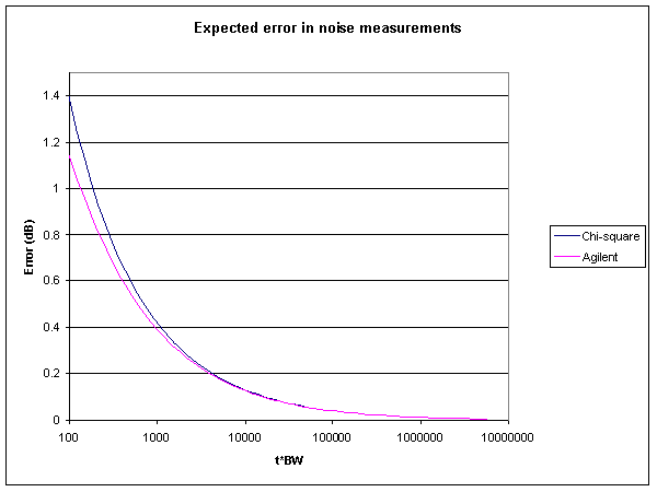 |
Fig 7 is a comparison of the chi-square estimate at confidence level 99.73% (equivalent to Normal distribution 3σ limits) with Agilent's expression. The difference is less than 0.01dB for t*BW>2700. Agilent's expression would appear to be an approximation of the chi-square estimate, and is reasonably accurate for t*BW greater than about 2000.
Agilent's approach may be based on a Normal approximation of Χ~χ2k for large k, but it appears to be a poor estimate for smaller k.
Glossary
| Term | Meaning |
| Aliasing | Distortion caused when the sample rate of a function (fs) is less than twice the highest frequency value of the input waveform or function. The frequencies above (fs/2) will be folded back into the lower frequencies. |
| Baseband | signals that contain a band of frequencies from zero and have a bandwidth of highest signal frequency. |
| dB | decibel - power ratio |
| dBm | decibels - power wrt 1 mW |
| Nyquist frequency | Half the sampling frequency of a discrete signal processing system (fs/2) |
| Nyquist Rate | The minimum sampling rate required to avoid aliasing, equal to twice the highest frequency contained within the signal (fs) |
Links
Noise measurement uncertainty calculator
FSM (Field Strength Meter) software
NFM (Noise Figure Meter) software
Theme page: Noise, LNA, Preamplifier, G/T, Receiver Performance
Changes
| Version | Date | Description |
| 1.01 | 28/06/2007 | Initial. |
| 1.02 | 24/03/09 | Added Agilent update. |
| 1.03 |