Category: Transmission lines

NanoVNA – interpolation – part 4 and prior articles discussed the possibility of significant error when calibration data is interpolated.

This article illustrates the effects with some very simple examples.

Test scenario

The test scenario is a NanoVNA-H4 with 5m length of RG58A/U to the reference plane. It has been OSL calibrated at the reference plane using a 1-101MHz 101 point sweep.

Result without interpolation of the calibration dataset

Above is a zoomed in view of 1-5MHz of a 1-101MHz 101 point sweep, there are measurements at every whole MHz value from 1 to 101. There are only 5 measurement points on this graph. Continue reading NanoVNA – interpolation – part 5

NanoVNA – interpolation – part 3 discussed selection of a sweep step size to provide sufficient data points for reasonably accurate interpolation.

When / where is interpolation used?

The VNA correction process uses measurements of some known conditions to create a calibration dataset, a table if you like of the sweep frequencies and calibration data. Commonly the calibration dataset is a table of the correction factors calculated from measurements of the knowns for each frequency of the calibration sweep. The correction factors are usually calculated for each frequency independently of adjacent frequencies.

When used to sweep a different range, interpolation can be used to interpolate those correction factors to the new measurement frequencies.

A common data flow is that shown above, where the correction terms are calculated for each of the frequencies in the calibration sweeps, and then those terms are interpolated to the frequencies actually used for a DUT measurement sweep. Continue reading NanoVNA – interpolation – part 4

NanoVNA – interpolation – part 3 discussed interpolation and introduced cubic spline interpolation.

NanoVNA-App v1.1.209-OD12 and prior used one of the special monotone types of cubic spline interpolation.

When used in VNA correction, the control points are often complex numbers with real and imaginary in broadly sinusoidal form and approximately 90° out of phase… so behavior on this scenario is important.

Above is a comparison of two types of interpolation on a pure sine wave. The green curve is the underlying sine curve, the orange dots are the samples or control points, the red curve is a linear interpolation, the blue dots are an example monotone cubic spline interpolation (monotone-cubic-spline.js). Continue reading NanoVNA-App v1.1.209-OD13 released

This article continues on from NanoVNA – interpolation – part 1 and NanoVNA – interpolation – part 2 which illustrated jagged scans at up to 900Mhz where the reference plane was displaced by 5m of RG58A/U.

A quite practical example where care must be taken is the following one at HF. Let’s say you wanted to measure the feed point impedance of some HF antenna, and the online gurus explained that one way to do that was to calibrate the NanoVNA and normal antenna coax feedline as a fixture, setting the reference plane to the feed point end of the coax.

A Simsmith model for illustration

A Simsmith model was constructed of a 30m (~100′) length of RG213 with a short circuit termination, and the real and imaginary parts of s11 as would be seen by the NanoVNA were plotted.

Let’s say you wanted to sweep from 1.5-33MHz (to include a little each side of the 160-10m bands… partly for reasons to be explained later.)

30m of RG213 @ 33MHz, step size 0.3MHz

Lets focus on the high frequency end where the jagged response is worse.

Again we see the periodic variation of s11 real and imaginary components as shown in the earlier articles. In the plot above, Simsmith as done a linear interpolation of the sweep points, and at 0.3MHz per step, the curves a jaggy. The actual minimum of the blue curve is at 33.88MHz, and the value is about 5% higher than the linear interpolation… which will introduce measurement noise to any VNA sweeps with such a configuration. Sweeps such as this are inputs to the calibration process. Continue reading NanoVNA – interpolation – part 3

NanoVNA – interpolation – part 1 introduced the principle on which VNA measurements are made and corrected based on a set of error terms derived from measurement of some known loads at the reference plane.

The technique of interpolation as a convenient means of increasing the utility and flexibility of a calibration data set was also introduced, and example raw (uncorrected) sweeps of an OC at the end of about 5m of RG58A/U were given to illustrate the challenge in interpolation with insufficient samples or control points.

A more common data flow is that shown above, where the correction terms are calculated for each of the frequencies in the calibration sweeps, and then those terms are interpolated to the frequencies actually used for a DUT measurement sweep. Continue reading NanoVNA – interpolation – part 2

A simple two port VNA allows measurement of  S parameters s11 and s21 of a DUT. Port 1 contains a directional coupler to transmit a signal into the DUT, and to capture and measure the amplitude and phase of the reflected wave relative to the forward wave at Port 1 (s11). Port 2 simply measures the amplitude and phase of the signal at its input, the forward wave after it has passed through the DUT relative to the forward wave at Port 1 (s21).

This is typically done by stepping (sweeping) the source on Port 1 through a range of frequencies, specified for example by start and end frequency and the number of discrete steps.

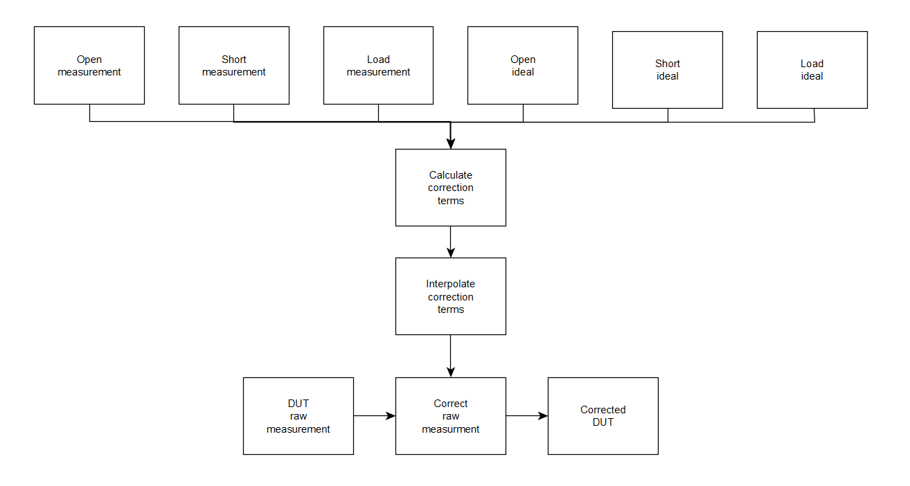
There are several source of error in such a measurement, but by making a series of measurements of some known configurations (Short, Open and Load on Port 1, Isolation and Through to Port 2), those errors can be determined and corrected out of subsequent measurements. So, there is a calibration process to measure and save measurements on these known loads, and then a correction process to apply the calculated corrections to raw measurements.

Early VNAs invalidated the calibration data if sweep parameters were changed, and so corrections were applied to raw measurements at corrections measured and calculated at exactly the same frequency.

This was really inconvenient, especially where no facility was provided to permanently save and restore a set of calibrations.

Later VNAs included the facility to interpolate (but not extrapolate) the calibration / correction data to a new set of sweep parameters. This was really convenient, but introduced a new source of error, the interpolation error.

When all this is done under the covers, users with little understanding of what is going on under the covers can easily obtain invalid / worthless results.

Let’s focus on s11 measurement, though the same issues exist for s21 measurement.

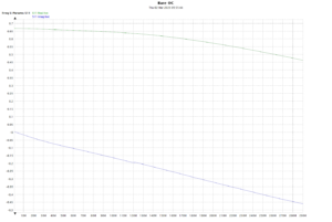
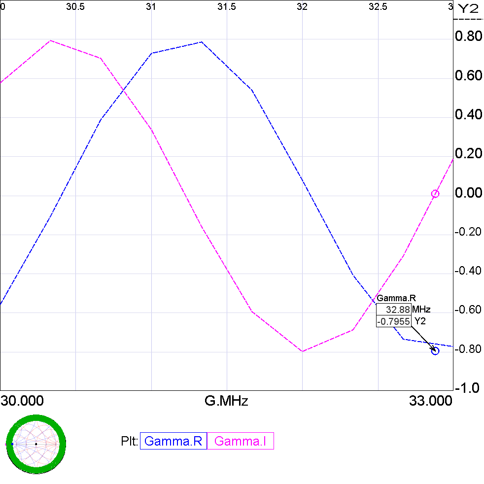
Above is a plot of uncorrected or raw s11 sweeping a NanoVNA-H4 101 points from 1 to 900MHz with nothing on Port 1 (approximately an open circuit OC). Ideally s11 should be 1+j0, but the directional coupler circuitry and small distance to the connector means the amplitude and phase vary as shown in the plot. Continue reading NanoVNA – interpolation – part 1

The usual method used for firmware upgrade is DFU (Direct Flash Update) using the USB interface and one of many PC clients to load the firmware.

Before attempting a firmware upgrade, be certain of the hardware you have, and the appropriate / compatible firmware file and format. Look for a label on the back, or on the silkscreen of the PCB (though sometimes hidden under the battery… doh!)… know what hardware you have to ensure you load compatible firmware.

Before discussing how to upgrade firmware if the USB interface is not functional, be sure that this problem is not driver related, that there is a real hardware problem. Continue reading nanoVNA-H – can firmware be updated if it has a broken USB socket?