Transmission lines – Page 41

Ratings of coax antenna switches

In a recent article I discussed how InsertionLoss implies InsertionVSWR in lossless devices.

This article looks at measurements of a few antenna switches at hand.

Daiwa CS-201G II

It is difficult to find comprehensive data on the very popular Daiwa CS-201 series switches.

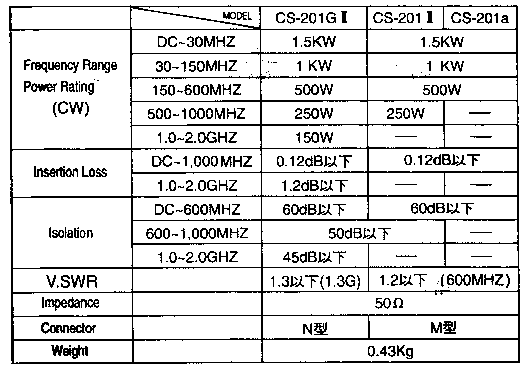
Above is the data from the packet of one of these switches, a CS-201G II. The specifications are pretty loose, and one must depend on one’s own measurements.

Above, the CS-201G II, a basic CS-201 series switch with N connectors, advertised as useful to 2000MHz where InsertionLoss is given as 1.2dB (or better?). If there were no TransmissionLoss in the switch, that would imply InsertionVSWR=3.6, but there is probably some significant TransmissionLoss and InsertionVSWR would be somewhat less. Nevertheless, IMHO InsertionLoss=1.2dB indicates it as unsuitable such frequencies. Continue reading Ratings of coax antenna switches

Last update: 5th July, 2016, 7:56 PM

InsertionLoss implies InsertionVSWR in lossless devices

Devices inserted in transmission lines often characterised by one or more of:

Insertion VSWR (the input VSWR when terminated with a matched load);
Return Loss (RL) in dB (20 times the log of the magnitude of the complex reflection coefficient); and
Insertion Loss.

Practitioners often find Insertion VSWR (1) of most use as it indicates whether the device is worse than other system devices, the weak link in the chain if you like. You might see a coax antenna switch specified to have InsertionVSWR<1.2 to 60MHz.

Return Loss (2) is a function of VSWR and vice versa, so it appeals when the designer thinks in terms of Return Loss rather than VSWR (and it is a better metric for VSWR<1.2). You might see a coaxial relay specified to have ReturnLoss>30dB to 500MHz.

Insertion Loss (3) is not so readily compared to the other two which are measures of input reflection with a matched termination. It often yields some numbers that appear very acceptable, but might be deceptively so. You might see a coaxial relay specified to have ReturnLoss>30dB to 500MHz. You might see a coax antenna switch specified to have InsertionLoss<0.2dB to 100MHz. Continue reading InsertionLoss implies InsertionVSWR in lossless devices

Last update: 12th October, 2023, 5:56 AM

Exploiting your antenna analyser #22

On a transmission line with standing waves, the voltage varies cyclically along the line, and is dependent also on power.

This article explains a method to use an analyser to predict the peak voltage level at a point for a given frequency and power based on measurement or estimation of complex Z or Y at that point using a suitable antenna analyser.

The problem

Lets say you have some critical voltage breakdown limit and want to use your analyser to find any non-compliance at the proposed power level.

Let us assume that the not-to-exceed voltage at that point is 1000Vpk. Let’s allow a little margin for variation due to factors not fixed, let’s actually use 800Vpk as the limit. We will use the maximum permitted power in Australia, 400W.
Continue reading Exploiting your antenna analyser #22

Last update: 30th June, 2016, 9:40 AM

End Fed Half Wave / Inverted L / Half Wave Dipole

The popular End Fed Half Wave is all things to all men, but this article compares an End Fed Half Wave, Inverted L, and Half Wave Dipole with some common parameters:

frequency: 7.1MHz;
flat top length: 20m;
Height above ‘average’ ground (σ=0.005, εr=13): 10m;
lossless balun / matching device.

Key differences:

ground connection: Inverted L = 2Ω, End Fed Half Wave = 100Ω; and
effective common mode choke used on the dipole.

Above is the modelled gain for all three. Continue reading End Fed Half Wave / Inverted L / Half Wave Dipole

Last update: 14th April, 2024, 1:36 PM

The magic of the End Fed Half Wave antenna / EFHW

I have noted recently the increasing popularity of the so-called End Fed Half Wave antenna, though the term often includes harmonic operation of the antenna.

It seems that at the heart of common ham understanding of this antenna system is that some kind of two terminal feed device creates a scenario with current on the nominal radiator, and zero common mode current on the feed line. If that feed device is small, its contents bears little influence on the current distribution on the feed line and radiator (the device behaviour approaches that of a simple circuit node).

Above is the kind of current distribution envisaged by many. The equivalent source is shown at the end fed feed point The red curve is the magnitude of current, the horizontal line represents the nominal radiator, and the vertical line represents the common mode conductor formed by the feed line. The feed line is often of arbitrary length, arbitrary route, and it may connect to real ground via an arbitrary impedance. Pretty much everything about this antenna system is random save the length of the nominal radiator. Continue reading The magic of the End Fed Half Wave antenna / EFHW

Last update: 14th April, 2024, 1:36 PM

Exploiting your antenna analyser #21

A correspondent wrote about the apparent conflict between Exploiting your antenna analyser #11 and Alan, K0BG’s discussion of The SWR vs. Resonance Myth. Essentially the correspondent was concerned that Alan’s VSWR curve was difficult to understand.

K0BG’s pitch

For convenience, here is the relevant explanation.

By definition, an antenna’s resonant point will be when the reactive component (j) is equal to zero (X=Ø, or +jØ). At that point in our example shown at left, the R value reads 23 ohms, and the SWR readout will be 2.1:1 (actually 2.17:1). If we raise the analyzer’s frequency slightly, the reactive component will increase (inductively) along with an increase in the resistive component, hence the VSWR will decrease, perhaps to 1.4:1. In this case, the MFJ-259B is connected to an unmatched, screwdriver antenna mounted on the left quarter panel, and measured through a 12 inch long piece of coax. This fact is shown graphically in the image at right (below).

Note that the graph is unscaled, and that frustrates interpretation. The text is also not very clear, a further frustration. It is easy to draw a graph… but is the graph inspired by a proposition or is it supporting evidence. Continue reading Exploiting your antenna analyser #21

Last update: 19th June, 2016, 7:12 PM

Exploiting your antenna analyser #20

Finding resistance and reactance with some low end analysers #2

Exploiting your antenna analyser #8 was about finding resistance and reactance with some low end analysers that don’t directly display those values of interest. The article showed how to calculate the values starting with |Z| from the analyser and included links to a calculator to perform the calcs.

This article describes an extension to that calculator Find |Z|,R,|X| from VSWR,|Z|,R,Ro to use R, VSWR, and Ro as the starting point. Note that the sign of X and the sign of the phase of Z cannot be determined from this starting point, there just isn’t enough information.

You will probably not find the equation for |X|(R,VSWR,Ro) in text books or handbooks, and the derivation is not shown here but if there is interest, I may publish a separate paper.

Lets say you knew VSWR=2, R=75Ω, Ro=50Ω, what is |X|?

Above, entering the values in the calculator we find that |X|=35.4Ω. Continue reading Exploiting your antenna analyser #20

Last update: 6th June, 2016, 8:09 AM

Analysis of a certain dipole animation – OCF implications

A correspondent having read Analysis of a certain dipole animation questioned the validity of the lossy transmission line model of the dipole, citing the case of an OCF half wave which has an approximately resistive feed point.

Since the OCF lacks the symmetry exploited in earlier study, we must consider each half of the OCF dipole and combine them. To assist, I have produced a similar plot of the transmission line but note the changed X axis.

The scenario is again a 2mm diameter copper wire, 3m above ground at 1MHz.

Z0 can be approximated as 138*log(2h/r)=138*log(2×3/0.001)=521Ω.

Above is a plot of calculated R,X components of V/I at displacements from the open end, and calculated phase of V/I. Continue reading Analysis of a certain dipole animation – OCF implications

Last update: 9th November, 2021, 10:33 AM

Exploiting your antenna analyser #19

Critically review your measurements

A recent post on an online forum provides a relevant example to discussion of this subject.

I have personally seen ratios similar to 3:1 or higher at the feed point become 1:1 at the rig over 100 or so feet of coax cable.

First point is that in good transmission line, it takes an infinite length to deliver the observations made above. Less might deliver almost VSWR=1 at the input end of the line.

Let us consider a practical scenario, 100′ of RG58A/U with a load of 150+j0Ω at 14MHz, the load end VSWR₅₀ is 3, the input impedance is 32.50-j22.86Ω and input VSWR₅₀ is 2.01. In this scenario, the line loss is 2.5dB which might be unacceptable for some applications. Continue reading Exploiting your antenna analyser #19

Last update: 21st May, 2016, 3:45 PM

Analysis of a certain dipole animation

Modern people look for videos and animations for their learning, and these are often not from reputable sources and raise more questions than they answer.

An example is an animation of a half wave dipole on the Internet, and being discussed on QRZ.

Above, the animated graphic.

Without trying to understand the problem, lets just extract two cases for further discussion, an analysis in the limits if you like. Continue reading Analysis of a certain dipole animation

Last update: 9th November, 2021, 10:31 AM