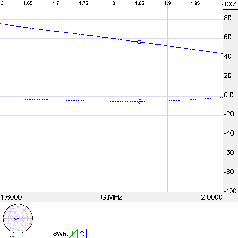
This article is a follow on from Receive only antenna for 160m – matching and performance discussion. It develops a SimNEC model that imports the loop impedance, and transforms it with an ideal transformer to quickly find an optimal transformer ratio and predict system losses.
Results are for the scenarios calculated and may not be extensible to different scenarios.
Another caveat: I have reservations about transmission line modelling in SimNEC, especially for composite conductors, but for the purposes of the discussion, assume that it is reasonably correct.
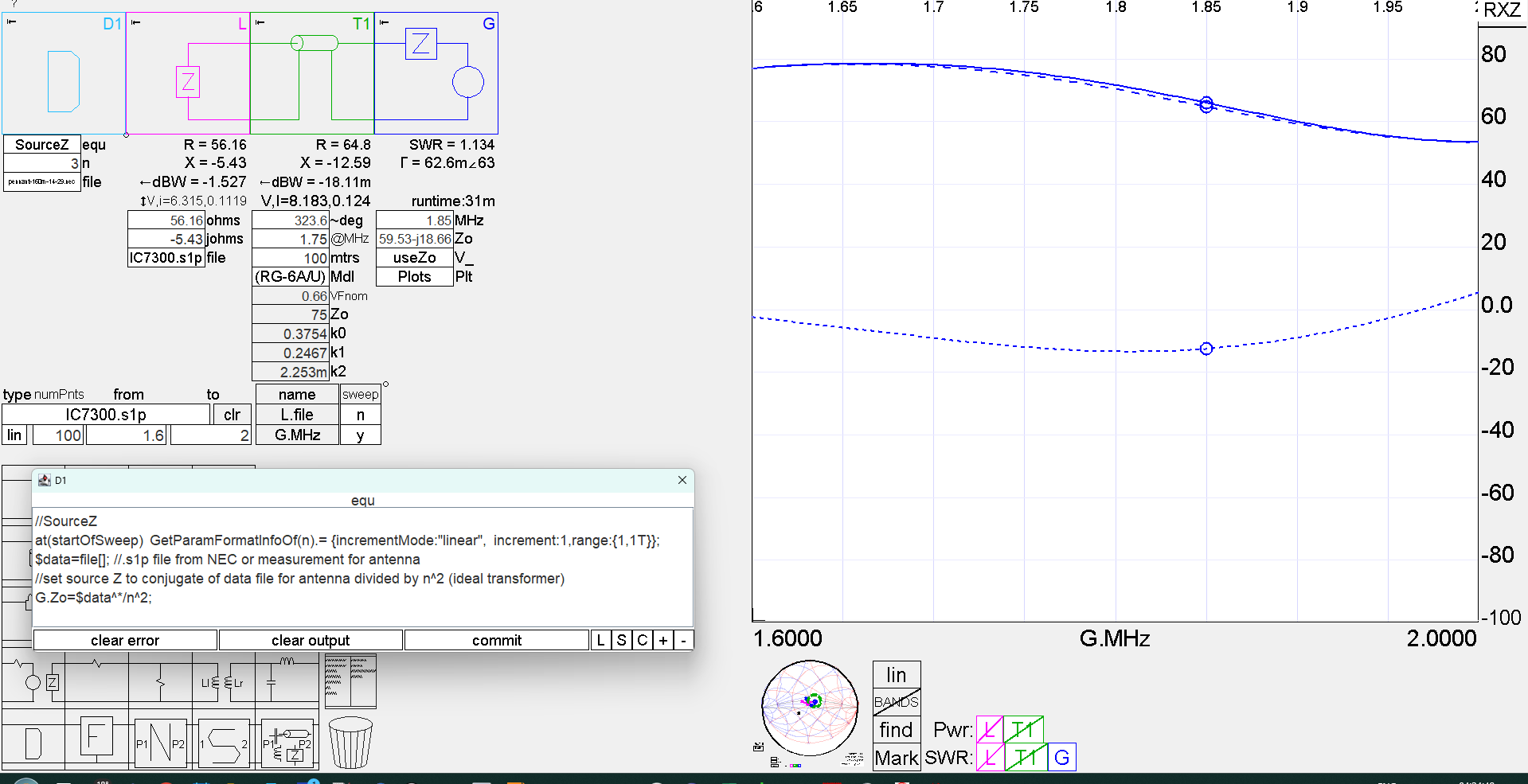
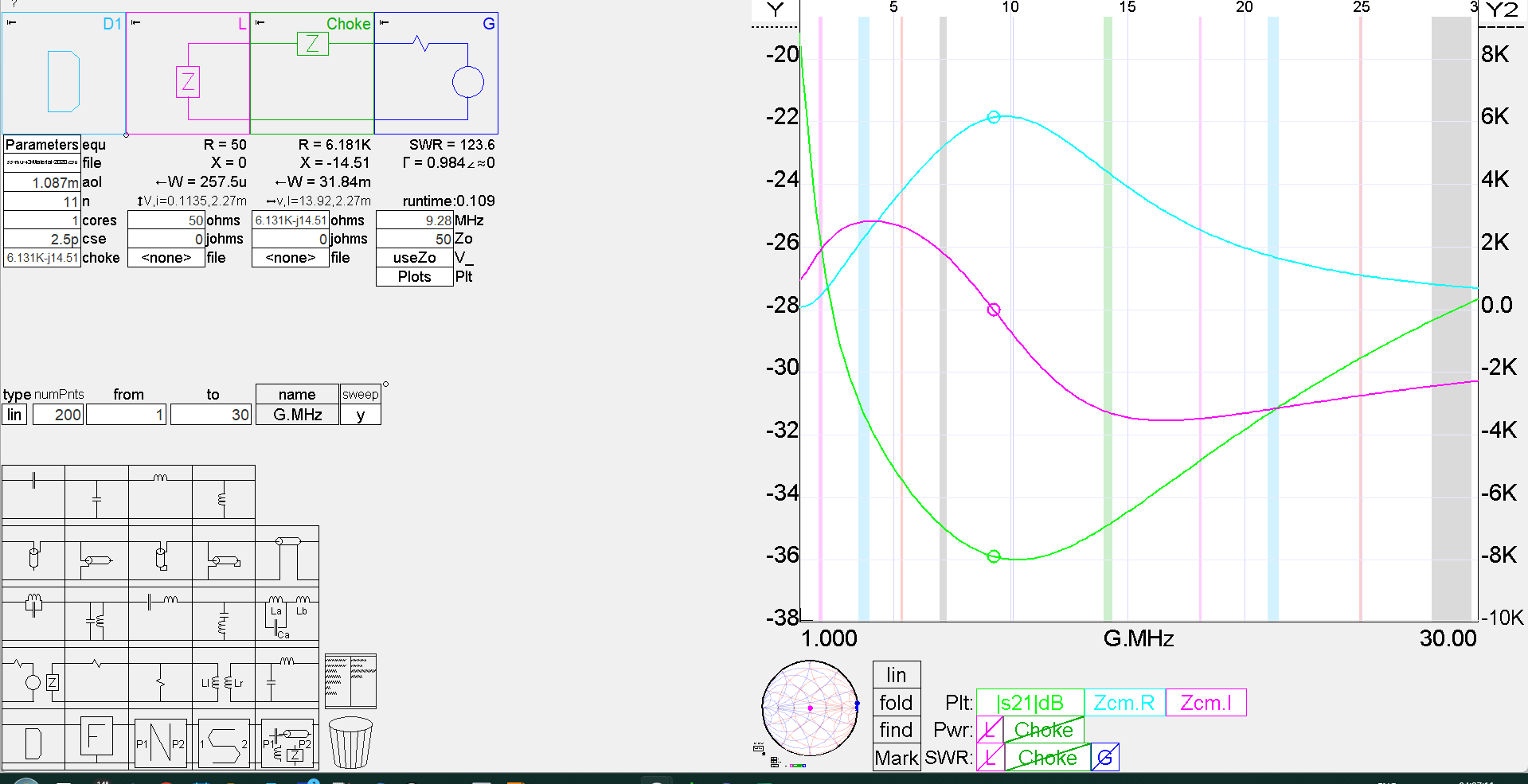
Above is the SimNEC model, it assumes reciprocity of the antenna system. Continue reading Receive only antenna for 160m – matching and performance discussion – improved SimNEC model