STL propaganda indeed: dipole – STL pattern comparison compared the patterns of a Inverted V dipole and STL, both configurations typical of SOTA deployments.
Seeing some pretty wild extrapolations to a vertical quarter wave with elevated radials, again typical of SOTA deployment, this article presents a comparison of all three using NEC-4.2 models.
See STL propaganda indeed and STL propaganda indeed: dipole – STL pattern comparison for details of the models for the STL and dipole.
The QW vertical is modelled using 2mm dia copper wire for vertical and radials, the radials are elevated 0.5m over ‘average ground’ (σ=0.005, εr=13).
Bear in mind that these are models that are based on some assumptions like ground parameters for example, and results may be different for other scenarios. Likewise, the results at 20m cannot simply be extrapolated to other bands, and practical modes of propagation utilised vary from band to band.
Key differences
Polarisation
Polarisation is a significant difference. Vertical ground waves are attenuated more slowly than horizontal waves, though ground wave propagation is not so commonly exploited on 20m due to its very short range. Because vertical ground waves are attenuated more slowly, a vertical polarised receiving antenna is likely to capture more ‘local’ noise that a horizontal one, but in SOTA context, local noise is not such an issue on mountain tops.
The QW vertical is vertical polarisation.
The STL is vertical polarisation.
The Inverted V dipole is horizontally polarised broadside to the dipole, and tends to vertical polarisation off the ends.
Radiation pattern
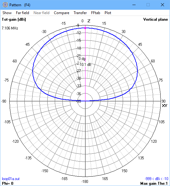
Radiation pattern is a 3 dimensional characteristic, often selectively plotted in two dimensions in the most favorable plane… which is fair enough but the reader needs to keep in mind the bigger three dimensional characteristic as it applies to their own application.
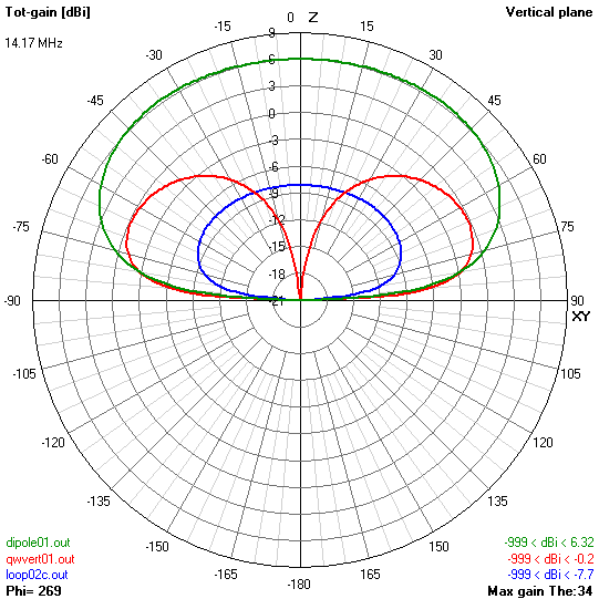
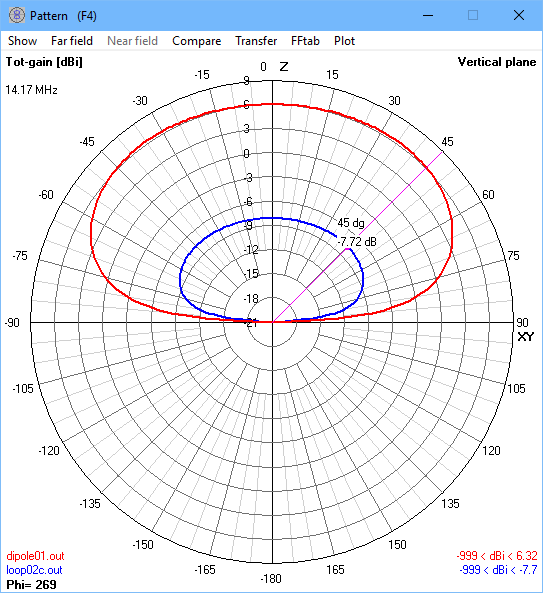
The radiation patterns of the antennas are quite different, the vertical is omnidirectional in azimuth whereas the others are not. So, it is challenging to produce a single general figure of merit comparing all antennas.

Above is a comparison of gain in the plane of maximum gain of the STL and dipole. Continue reading STL propaganda indeed: QW vertical – dipole – STL model pattern comparison
Last update: 3rd July, 2017, 10:38 AM
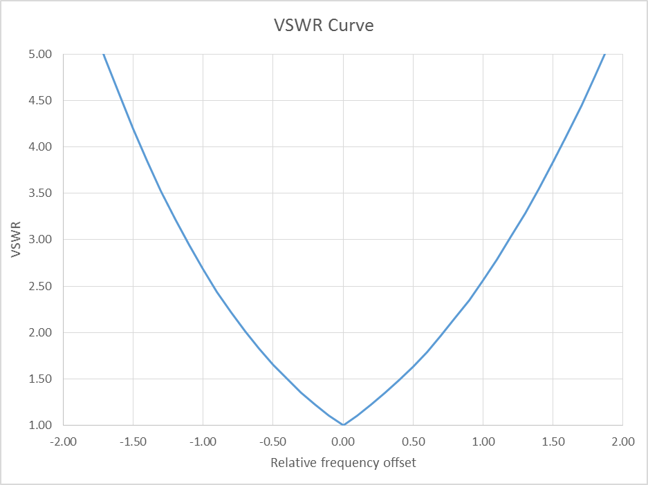
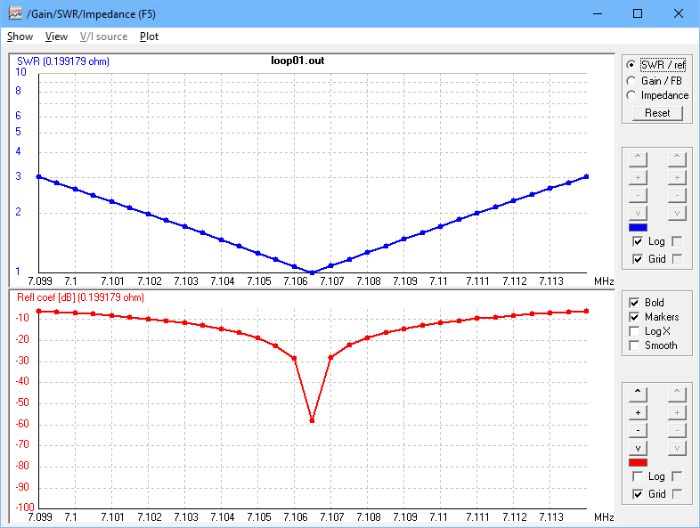
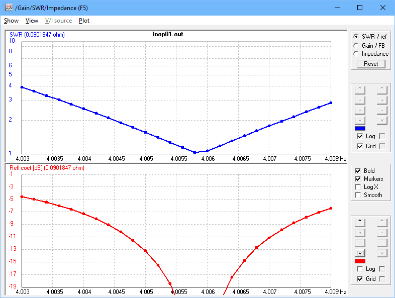
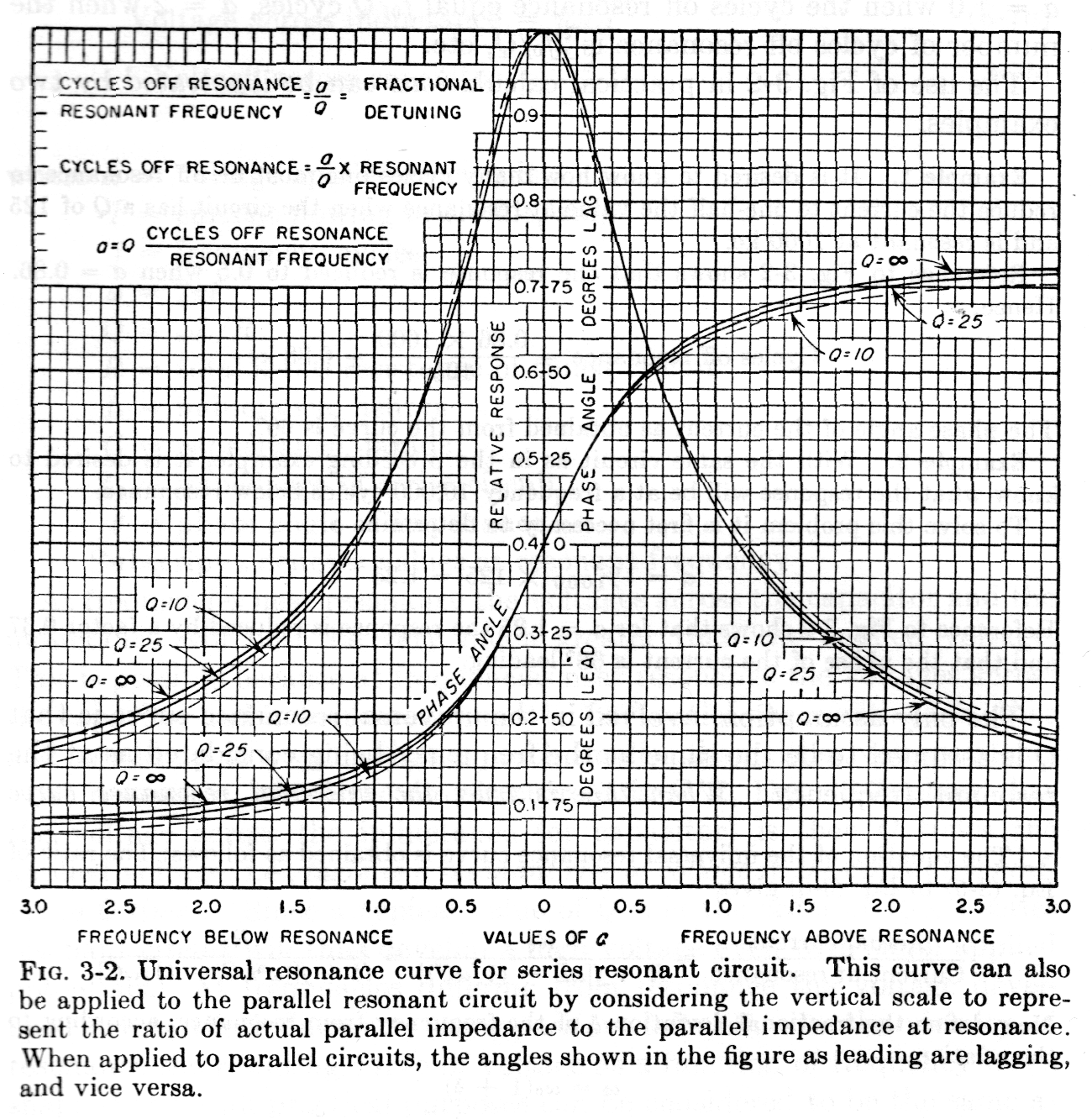 Above is a chart of the Universal Resonance Curve from (Terman 1955). The chart refers to “cycles”, the unit for frequency before Hertz was adopted, and yes, these fundamental concepts are very old. Continue reading Antenna half power bandwidth and Q, concept and experimental validation