NEC model of figure 8 transmitting loop

Variants of loops have been designed and promoted as having certain advantages, and one of those is the so-called figure 8 loop.

This article describes an NEC-4.2 model at 14MHz of an antenna similar to a commercial example.

The graphic shows the geometry. In this case the source is at the bottom of the lower loop, and the blue square is the tuning capacitor. The loop conductor is 22mm copper tube, the loop diameters are 1m, and the capacitor connection is 100mm wide. Commonly these are fed by a low loss auxiliary loop at the bottom of the lower loop, but the direct feed is quite fine for modelling the loop performance. Continue reading NEC model of figure 8 transmitting loop

The system wide conjugate match stuff crashes out again

Walt Maxwell (W2DU) made much of conjugate matching in antenna systems, he wrote of his volume in the preface to (Maxwell 2001 24.5):

It explains in great detail how the antenna tuner at the input terminals of the feed line provides a conjugate match at the antenna terminals, and tunes a non-resonant antenna to resonance while also providing an impedance match for the output of the transceiver.

Walt Maxwell made much of conjugate matching, and wrote often of it as though at some optimal adjustment of an ATU there was a system wide state of conjugate match conferred, that at each and every point in an antenna system the impedance looking towards the source was the conjugate of the impedance looking towards the load.

This was recently cited in a discussion about techniques to measure high impedances with a VNA:

WHEN the L and C’s of the tuner are set to produce a high performance return loss as measured by the vna, then in essence, if the tuner were terminated (where the vna was positioned) with 50 ohms and we were to look into the TUNER where the antenna was connected, we would see the ANTENNA Z CONJUGATE. Wow, that’s a mouth full. The best was to see this is to do an example problem and a simulator like LT Spice is a nice tool to learn. Or there are other SMITH GRAPHIC programs that are quite helpful to assist in this process. Standby and I will see what I can assemble.

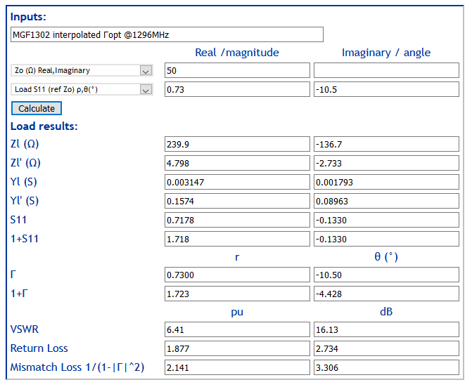
The example subsequently described set about demonstrating the effect. The example characterised a certain antenna as having an equivalent circuit of 500Ω resistance in series with 4.19µH of inductance and 120pF of capacitance (@ 7.1MHz, Z=500-j0.119, not quite resonant, but very close). A lossless L network (where do you get them?) was then found that gave a near perfect match to 50+j0Ω. The proposition is that if you now look into the L network from the load end, that you see the complex conjugate of the antenna, Z=500+j0.119.

I asked where do you get a lossless L network? Only in the imagination, they are not a thing of the real world. Continue reading The system wide conjugate match stuff crashes out again

RG6/U with CCS centre conductor at HF

At Series match for a half wave dipole I mentioned that RG6/U may have a copper clad steel (CCS) centre conductor, and may have significantly more loss at HF than expected based on datasheets and calculators.

Above is a comparison of matched line loss based on measurement of a length of RG6/U Quad Shield CCS cable and prediction from Simsmith of Belden 8215 (also CCS). The ripple is due to measurement system error. Continue reading RG6/U with CCS centre conductor at HF

Series match for a half wave dipole

An online poster was demonstrating the effect of varying line length on a half wave dipole on VSWR50 and by mistake configured the line be of of Zo=75Ω.

He asked the question

In the general case, if you are trying to match 50 Ohms, would you be better off feeding a normal backyard dipole with 75 Ohm coax if you are willing to prune it to a specific length after the fact?

Continue reading Series match for a half wave dipole

Rigexpert AA-600 reference plane

The Rigexpert AA-600 has an inbuilt calibration which is convenient to use. It is capable of OSL calibration, but this article discusses only the inbuilt calibration.

The reference plane is the plane at which the instrument calibration is correct, at other locations there is a transmission line impedance transformation applied.

The pic above shows the reference plane, but where exactly is it and why do you want to know? Continue reading Rigexpert AA-600 reference plane

SimSmith – looking both ways – an LNA design task

This article shows the use of SimSmith in design and analysis of the input circuit of an MGF1302 LNA.

The MGF1302 is a low noise GaAs FET designed for S band to X band amplifiers, and was very popular in ham equipment until the arrival of pHEMT devices.

An important characteristic of the MGF1302 is that matching the input circuit for maximum gain (maximum power transfer) does not achieve the best Noise Figure… and since low noise is the objective, then we must design for that.

The datasheet contains a set of Γopt for the source impedance seen by the device gate, and interpolating for 1296MHz Γopt=0.73∠-10.5°.

Lets convert Γopt to some other useful values.

The equivalent source Z, Y and rectangular form of Γopt= will be convenient during the circuit design phase. Continue reading SimSmith – looking both ways – an LNA design task

Transmitter / antenna systems and the maximum power transfer theorem

Jacobi’s Maximum Power Transfer Theorem

Jacobi’s law (also known as Jacobi’s Maximum Power Transfer Theorem) of nearly 200 years ago stated

Maximum power is transferred when the internal resistance of the source equals the resistance of the load.

Implied is that the internal resistance of the source is held constant, it does not work otherwise. The source must be one that can validly be represented by a Thevenin equivalent circuit. This was in the very early days of harnessing electric current, direct current initially.

Later adaptation dealt with alternating current and it became

Maximum power is transferred when the load impedance is equal to the complex conjugate of the internal impedance of the source.

Again a necessary condition is that the source must be one that can validly be represented by a Thevenin equivalent circuit. Continue reading Transmitter / antenna systems and the maximum power transfer theorem

Walter Maxwell’s teachings on system wide conjugate matching – a SimSmith example

I have written on Walt Maxell’s proposition about simultaneous system wide conjugate matching in antenna systems. I will repeat a little to set the context…

Walt Maxwell (W2DU) made much of conjugate matching in antenna systems, he wrote of his volume in the preface to (Maxwell 2001 24.5):

It explains in great detail how the antenna tuner at the input terminals of the feed line provides a conjugate match at the antenna terminals, and tunes a non-resonant antenna to resonance while also providing an impedance match for the output of the transceiver.

Walt Maxwell made much of conjugate matching, and wrote often of it as though at some optimal adjustment of an ATU there was a system wide state of conjugate match conferred, that at each and every point in an antenna system the impedance looking towards the source was the conjugate of the impedance looking towards the load.

This is popularly held to be some nirvana, a heavenly state where transmitters are “happy” and all is good. Happiness of transmitters is often given in online discussion by hams as the raison d’être for ATUs, anthropomorphism over science. Continue reading Walter Maxwell’s teachings on system wide conjugate matching – a SimSmith example

Franklin antenna – how does it work?

(Franklin 1924) described a technique to cophase sections of a long antenna by “concentrating alternating half wave length portions of the wire within a small space, by winding such portions as inductance coils or by doubling such portions back on themselves so that there is practically no radiation from these portions”.

Let’s explore his second option, as unlike the first, it does work reliably.

Above is an NEC-4.2 model with current shown (magnitude and phase). The stubs conductors are all defined from top to bottom. Continue reading Franklin antenna – how does it work?