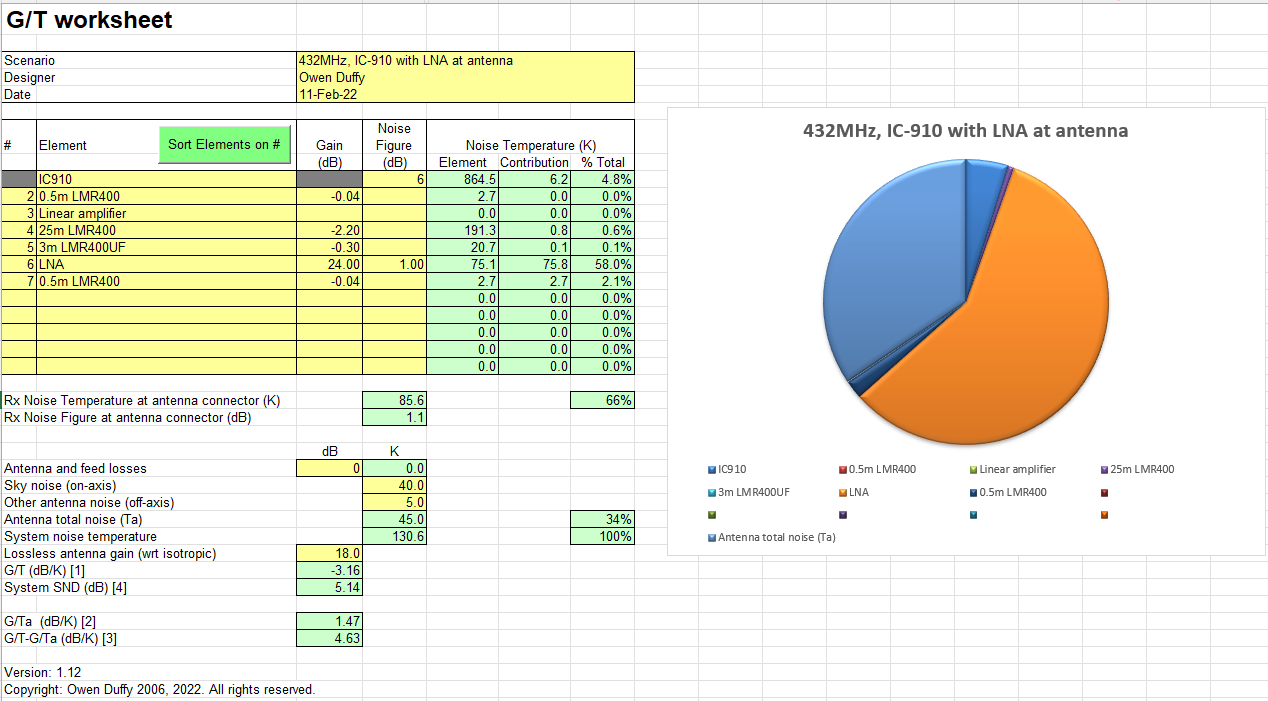
For those who may have used or want to use my G/T spreadsheet tool I have released an improved version 1.12. This is not a bug fix. Continue reading G/T spreadsheet update (v1.12)
For those who may have used or want to use my G/T spreadsheet tool I have released an improved version 1.12. This is not a bug fix. Continue reading G/T spreadsheet update (v1.12)
By broadband transformer, I mean a transformer intended to have nearly nominal impedance transformation over a wide frequency range. That objective might be stated as a given InsertionVSWR over a given frequency range for a stated impedance. eg InsertionVSWR<2 from 3-30MHz with 3200(+j0)Ω load.
These are used in many things, including medium to high power applications such as EFHW matching transformers.
Leakage inductance is the equivalent series inductance due to flux that cuts one winding and not the other, and vice versa. For most simple transformers, the total primary referred leakage inductance is twice the primary leakage inductance. Since the leakage inductance appears in series with the signal path, it causes degradation of nominal impedance transformation, the very simplest approximation of the frequency response is that of a LR circuit.
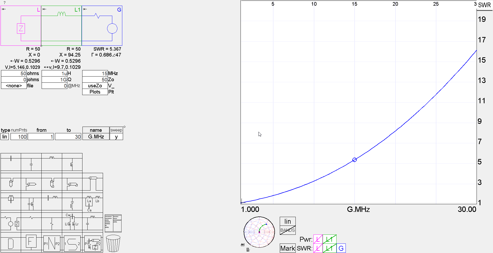
Above is a Simsmith model of a 1µH total leakage inductance in series with a 50+j0Ω load, the InsertionVSWR is greater than 1.5 above 3MHz.
Is this a common scenario? Continue reading On ferrite cored RF broadband transformers and leakage inductance
Over more than 50 years, I have measured literally thousands of RF inductors and transformers. This article gives some hints and techniques for making / preparing prototypes for measurement, and measurement.
RF inductors and transformers will often use enameled copper wire (ECW) or some form of insulated wire or coax.
Solid core LAN cables are a good source of small insulated wire for prototyping. The conductor is around 0.5mm, and overall about 0.9mm.
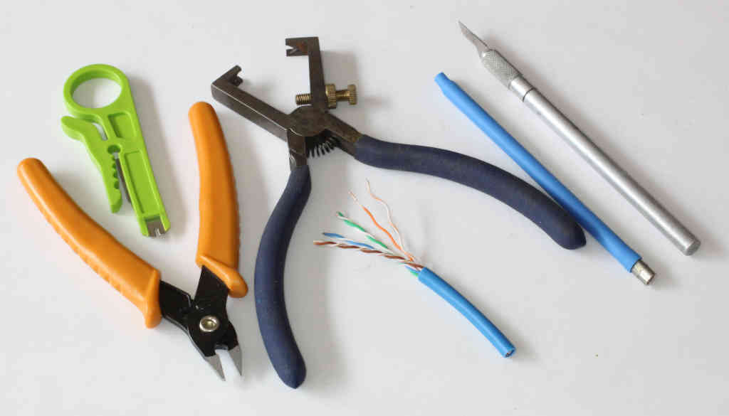
Above, from left to right: Continue reading Tips and techniques for measuring small RF inductors and transformers
A common scheme for narrow band match of an end fed high Z antenna gives a Simsmith model for the matching arrangement that follows.
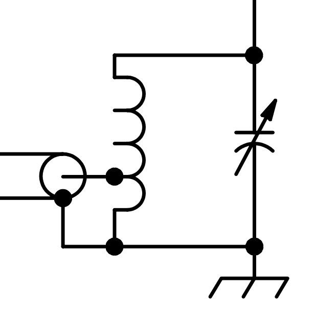
The tapped coil could also be considered an autotransformer.
I have owned a NanoVNA-H v3.3 for more than two years now. It required some modification to fix a power supply decoupling problem on the mixers, reinforcement of the SMA connectors, replacement of the USB socket, rework of the case so the touch screen worked properly / reliably, and some minor works (eg battery charger chip, bad patch cables, faulty USB cable).
With recent enhancement of firmware to support an SD card, the prospect of stand alone use becomes more practical, so I set about researching and purchase.
It seemed the best option was to buy a ‘genuine’ NanoVNA-H4 v4.3, and I started the search at the recommended (by Hugen) store, Zeenko… but whilst there was a listing for v4.2, there was no v4.3 listing (perhaps it is out of stock). I did find another store selling what they described as a ‘genuine’ NanoVNA-H4 v4.3, but this is a high risk transaction, experience is that Chinese sellers are not to be trusted, and Aliexpress is an unsafe buying platform.
This is one of those concerning transactions where the seller notifies shipment and gives a tracking number hours before the deadline, then a week later change the tracking number (the ‘real’ shipment).

Above, the promo image from the listing. Continue reading NanoVNA-H4 v4.3 – initial impressions
This article describes a method of measurement and adjustment using an antenna analyser or VNA to quickly set up a shunt match, a narrow band match (ie for one band, or even only part of the band).
The article uses Rigexpert’s Antscope as the measurement / analysis application, the techniques will work with other good application software.
To demonstrate the technique for matching such an antenna, let’s use NEC-4.2 to create 80m feed point impedance data for a 12m high vertical with 8 buried radials (100mm) and centre loading coil resonating the antenna in the 80m band for simulation of measurement data.
An s1p file was exported from 4NEC2 for import into Antscope, to simulate measurement of an example real antenna.
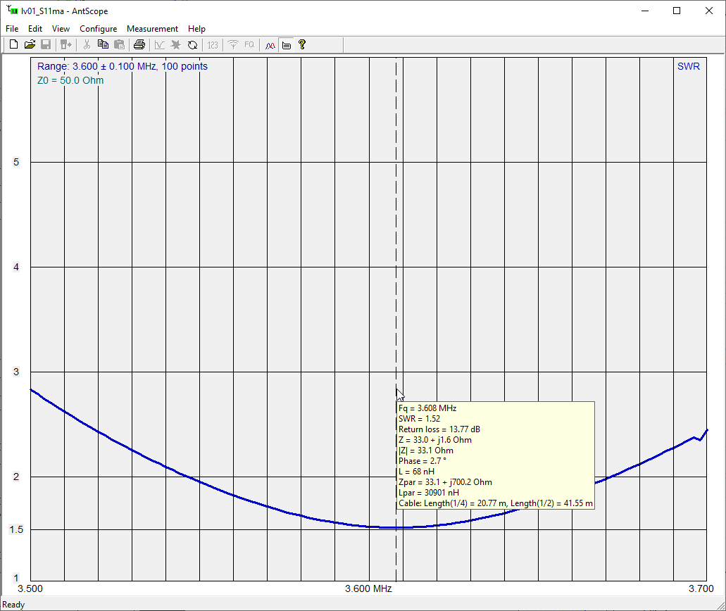
Above is the VSWR curve displayed in Antscope. Note that the actual response is dependent on soil types, antenna length and loading etc, but this is a good example for discussion. It is not real bad, another example might be better or worse. Continue reading Matching a centre loaded 80m vertical – a shunt match tutorial
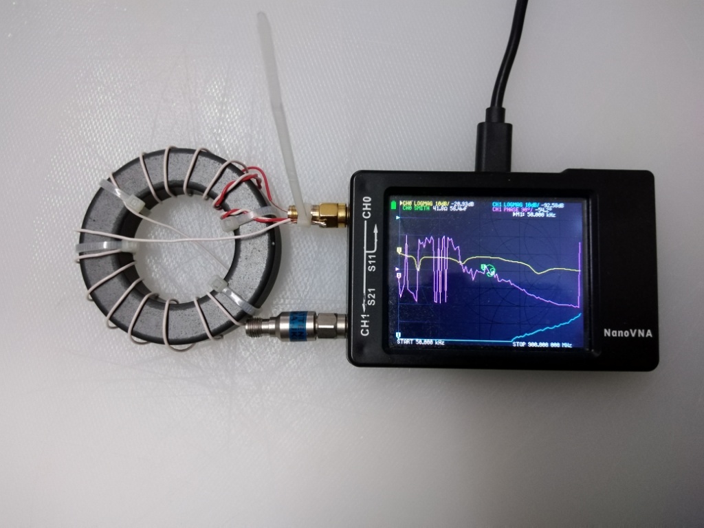
It seems that lots of hams find measuring the impedance of a common mode choke a challenge… perhaps a result of online expert’s guidance?
The example for explanation is a common and inexpensive 5943003801 (FT240-43) ferrite core.
It helps to understand what we expect to measure.
See A method for estimating the impedance of a ferrite cored toroidal inductor at RF for an explanation.
Note that the model used is not suitable for cores of material and dimensions such that they exhibit dimensional resonance at the frequencies of interest.
Be aware that the tolerances of ferrite cores are quite wide, and characteristics are temperature sensitive, so we must not expect precision results.
Above is a plot of the uncalibrated model of the expected inductor characteristic, it shows the type of response that is to be measured. The inductor is 11t wound on a Fair-rite 5943003801 (FT240-43) core in Reisert cross over style using 0.5mm insulated copper wire. Continue reading nanoVNA – measure common mode choke – it is not all that hard!
EFHW-2843009902-43-2020-3-6kThis article applies the Simsmith model described at A simple Simsmith model for exploration of a common EFHW transformer design – 2t:14t to a ferrite cored 50Ω:200Ω transformer.
This article models the transformer on a nominal load, being \(Z_l=n^ 2 50 \;Ω\). Keep in mind that common applications of a 50Ω:200Ω transformer are not to 200Ω transformer loads, often antennas where the feed point impedance might vary quite widely, and performance of the transformer is quite sensitive to load impedance. The transformer is discussed here in a 50Ω:200Ω context.
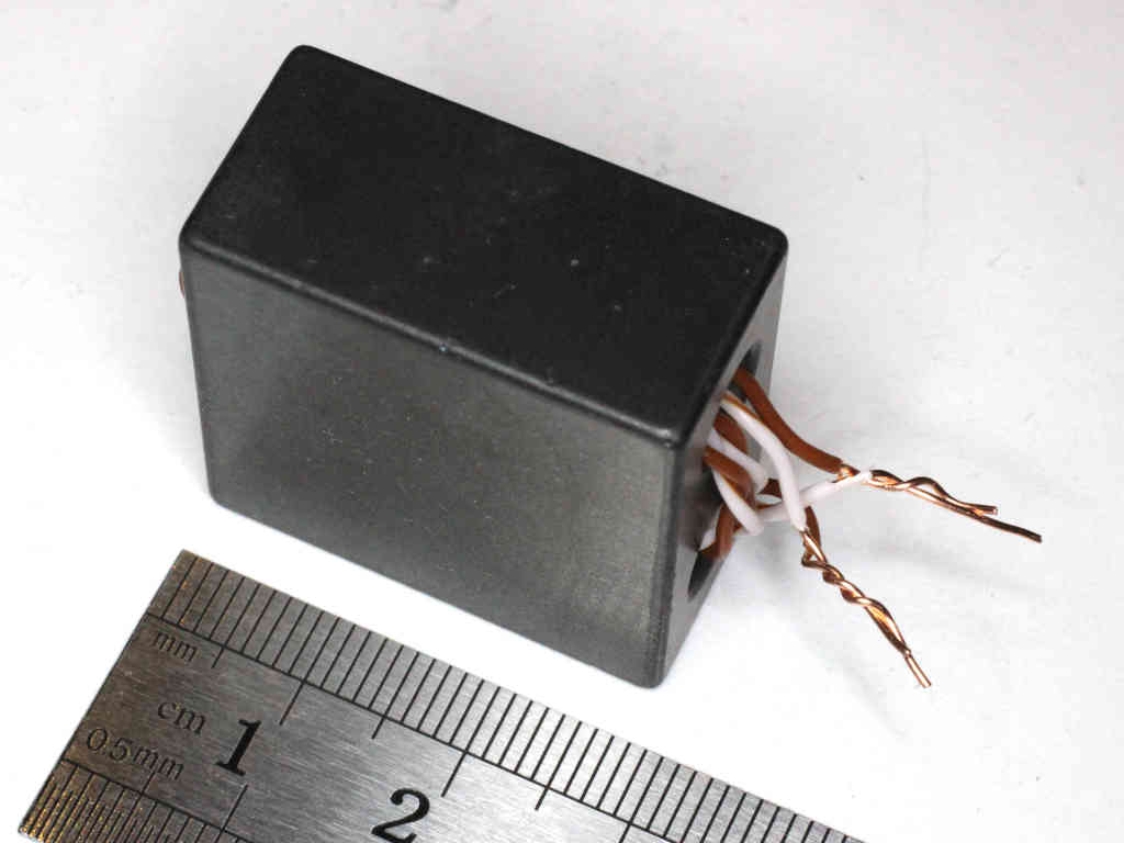
Above is the prototype transformer using a 2843009902 (BN43-7051) binocular #43 ferrite core, the output terminals are shorted here, and total leakage inductance measured from one twisted connection to the other. Continue reading A simple Simsmith model for exploration of a 50Ω:200Ω transformer using a 2843009902 (BN43-7051) binocular ferrite core
This article describes a Simsmith model for an EFHW transformer using a popular design as an example.
This article models the transformer on a nominal load, being \(Z_l=n^ 2 50 \;Ω\). Real EFHW antennas operated at their fundamental resonance and harmonics are not that simple, so keep in mind that this level of design is but a pre-cursor to building a prototype and measurement and tuning with a real antenna.
Above is the prototype transformer measured using a nanoVNA, the measurement is of the inductance at the primary terminals with the secondary short circuited. Continue reading A simple Simsmith model for exploration of a common EFHW transformer design – 2t:14t
This article describes a Simsmith model for an EFHW transformer using a popular design as an example.
This article models the transformer on a nominal load, being \(Z_l=n^ 2 50 \;Ω\). Real EFHW antennas operated at their fundamental resonance and harmonics are not that simple, so keep in mind that this level of design is but a pre-cursor to building a prototype and measurement and tuning with a real antenna.
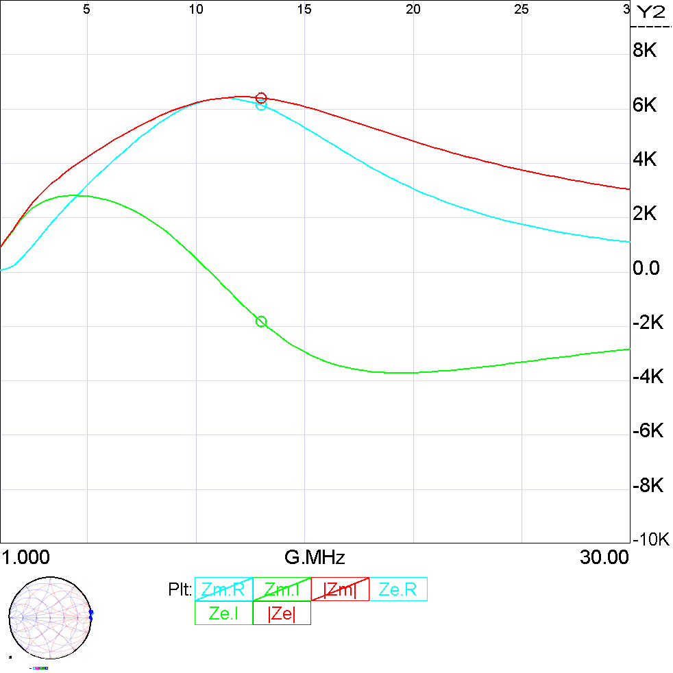
The prototype transformer follows the very popular design of a 2:16 turns transformer with the 2t primary twisted over the lowest 2t of the secondary, and the winding distributed in the Reisert style cross over configuration.
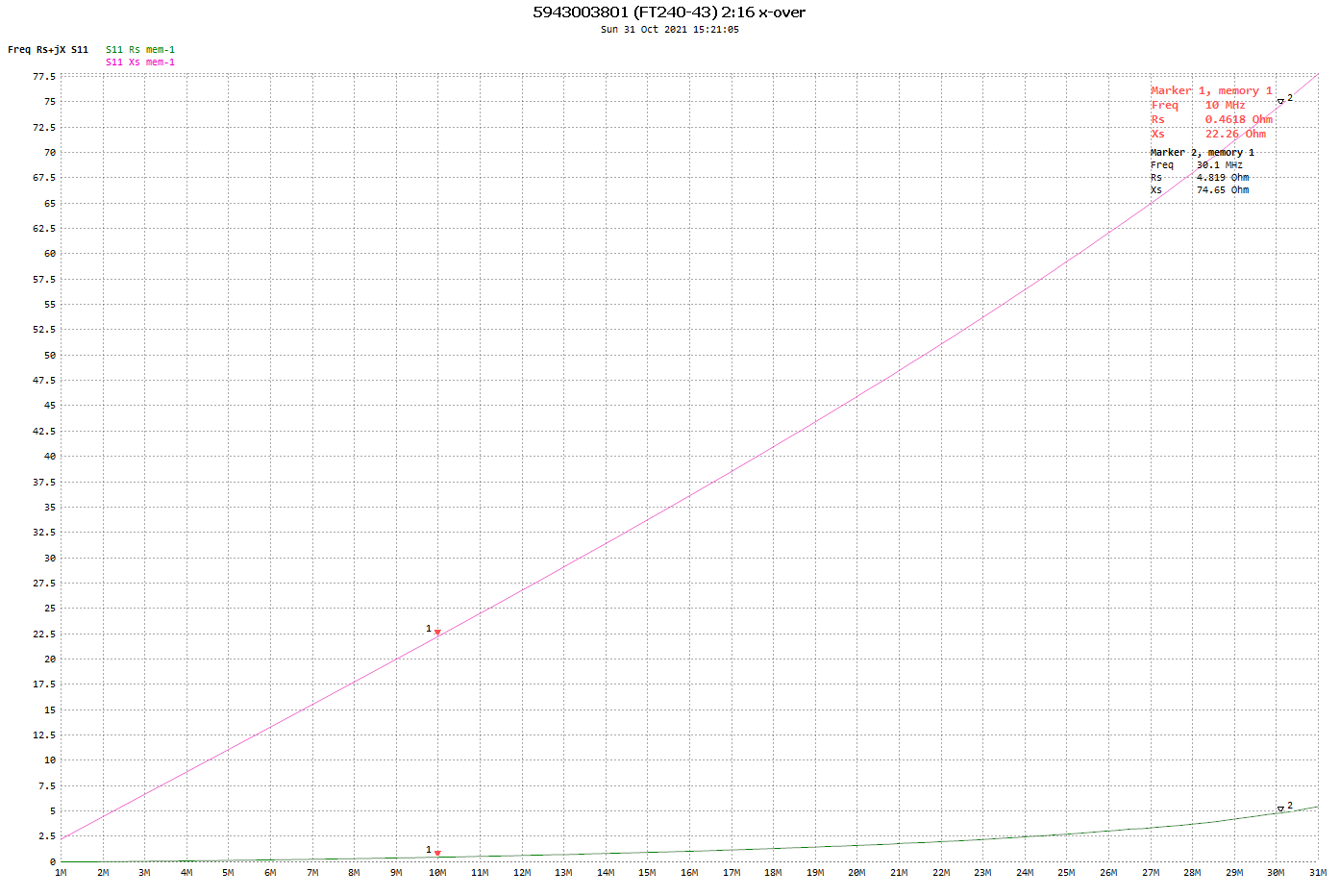
Above is a plot of the equivalent series impedance of the prototype transformer with short circuit secondary calculated from s11 measured with a nanoVNA from 1-31MHz. Note that it is almost entirely reactive, and the reactance is almost proportional to frequency suggesting close to a constant inductance. Continue reading A simple Simsmith model for exploration of a common EFHW transformer design – 2t:16t