Frank, W3LPL conducted two interesting experiments with WSPRlites on 20m from the US to Europe essentially. This article discusses the first test.
The first experiment was a calibration run if you like to explore the nature of simultaneous WSRP SNR reports for two transmitters using different call signs on slightly different frequencies (19Hz in this case) feeding approximately the same power to the same antenna.
The first test uses two WSPRlites feeding the same antenna through a magic-T combiner producing a data set consisting of 900 pairs of SNR reports from Europe with only about 70 milliwatts from each WSPRlite at the antenna feed.
The data for the test interval was extracted from DXplorer, and the statistic of main interest is the paired SNR differences, these are the differences in a report from the same station of the two signals in the same measurement WSPR interval.
There is an immediate temptation of compare the average difference, it is simple and quick. But, it is my experience that WSPR SNR data are not normally distributed and applying parametric statistics (ie statistical methods that depend on knowledge of the underlying distribution) is seriously flawed.
We might expect that whilst the observed SNR varies up and down with fading etc, that the SNR measured due to one transmitter is approximately equal to that of the other, ie that the simultaneous difference observations should be close to zero in this scenario.
What of the distribution of the difference data?
Above is a frequency histogram of the distribution about the mean (0). Interpretation is frustrated by the discrete nature of the SNR statistic (1dB steps), it is asymmetric and a Shapiro-Wik test for normality gives a probability that it is normal p=1.4e-43.
So lets forget about parametric statistics based on normal distribution, means, standard deviation, Student’s t-test etc are unsound for making inferences because they depend on normality.
Nevertheless, we might expect that there is a relationship between the SNR reports for both transmitters, We might expect that SNR_W3GRF=SNR_W3LPL.
So, lets look at the data in a way that might expose such a relationship.
Above is a 3D plot of the observations which shows the count of spots for each combination of SNR due to the two transmitters. The chart shows us that whilst there were more spots at low SNR, the SNRs from both are almost always almost the same.
A small departure can be seen where a little ridge exists in front of the main data.
Lets look at in 2D.
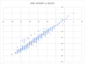
Above is a 2D chart of the same data. Note that there are 902 observations, so many of the dots account for scores of observations as can be seen in the 3D chart above.
The outliers can be seen more clearly, but it isn’t so obvious that there is only a small number of them. In fact, examining the data showed that the outliers came from only one observer, and all of their observations (about 15) were outliers. There is a strong case to exclude them as anomalous.
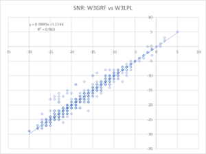
Above after stripping the 15 anomalous records, there is an obvious trend. Above, we have used Excel to add a linear trend line to the data. Remember that individual dots may account for scores of observations, all observations are used to calculate the trend line.
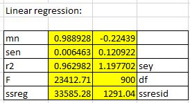
Above is a more detailed regression result using Excel’s LINEST() function.
The coefficients tell us that the slope of the curve fit is almost exactly 1 (0.9975) and so the system appears quite linear over the range tested. The intercept is -0.1684 with, it is the difference in SNR between the two transmitters and as might be expected it is fairly close to zero.
Data quality
Data obtained for any experiment needs careful review. There are a host of problems which influence WSPR data quality, some inherent in the system, some related to the end stations, some in the data archive. In my experience, WSPR data deserves great more attention to identify and excise anomalous records.
The experiment described here assumes a single ‘spot’ record lodged by each station hearing each of the transmitters and is spoiled if there is more than a single record for each. It has been observed that there can be more than a single record (eg if a call sign was simultaneously active on more than one receiver on that frequency), and those records should be excised to improve data quality (DXplorer contains a facility to do that and an override switch).
Conclusions
- The observed SNR difference was not normally distributed and therefore unsuitable for parametric statistical analysis based on normal distribution.
- Careful examination of the data highlighted a very small number of outliers which were excised to improve the model quality.
- A linear regression is a non-parametric analysis that produced a very low error model explaining the dataset.
- The actual power output of each transmitter was not measured but estimated and that contributes to measured SNR difference.
- The test results were that the differences between simultaneous measurements of SNR for each transmitter at a number of observing stations was -0.24dB with standard error of 0.1dB.
- The results are quite consistent with almost equal transmitters feeding the same antenna, and suggest that the method might lend itself to comparison of two different antennas using two WSPRlites.


