Estimating parameters of two wire transmission lines

Hams often construct two wire transmission lines from available material. In many applications, the characteristic impedance (Zo) is not particularly critical, in others it may be an important parameter of an impedance matching scheme. Likewise, the attenuation characteristic, and particularly loss with a mismatched load may be important.

Traditional method

The traditional method is to regard the line loss as so low that it can be treated as lossless. Characteristic impedance is often calculated as 276log(s/r) where s is the centre to centre spacing and r is the radius of the conductors. Velocity factor (vf) is usually taken to be one;

Let's try an example. Using TET-EMTRON's line spacers and the recommended 2mm diameter stranded copper wire, s=50 and r=1 so Zo=469Ω.

This method is flawed for several reasons:

• the approximation 276log(s/r) falls down for small ratios s/r;
• velocity factor is rarely so close to unity to be taken as that;
• lines are never lossless, and some dielectrics in cables not intended as RF transmission lines can be significant even at HF.

A better model

The expression Zo=120acosh(D/d) is a better one, though at very close spacings, proximity effect introduces significant error.

So, to calculate the above example still assuming vf=1, Zo=469.40-j1.05Ω, Not a lot different in this case, but the reactive component is a result of inclusion of the conductor loss.

But the velocity factor of a practical line is not 1, the materials used to maintain the uniform spacing of the conductors reduces the velocity factor and introduces some dielectric loss.

Factoring in the spacers and adjusting the permittivity to deliver the measured velocity factor, Zo=453.78-j1.01Ω. Using more or less spacers per unit length will affect vf and Zo to some extent.

Now that a better estimate of Zo, and the R and G terms of the RLGC transmission line model have been estimated, matched line loss can be calculated at a given frequency. The matched line loss for 10m of this line at 3.7MHz is calculated as 0.0156dB (or 0.156db/100m). This might seem essentially lossless, but if it were used to feed a load of 9.7-j337Ω (such as likely with a G5RV), then the loss with that load is 0.912dB. Thought it is not extreme, it is much higher than the matched line loss, almost 60 times the dB value.

Taking one popular windowed ladder line, Wireman 551 as another example. If it used solid copper conductors for the same electrical length, it would have a 1.55dB mismatched loss, but it probably doesn't, it uses copper clad steel and the copper cladding is not sufficiently thick to assure copper like performance at 3.7MHz, so actual loss is probably higher.

The RLGC transmission line model

Fig 1:

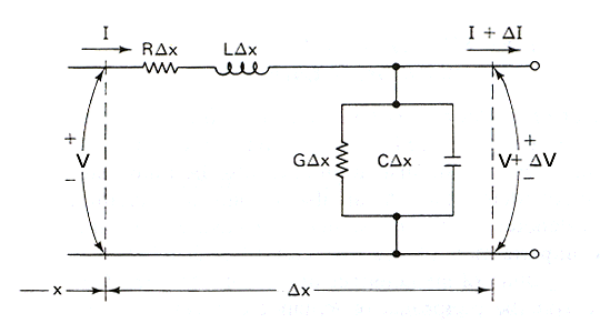
A transmission line can be represented as an infinite series of cascaded identical two port networks each representing an infinitely small section of the transmission line. The small networks represent:

• the distributed resistance of the conductors is represented by a series resistance per unit length R;
• the distributed inductance is represented by a series inductance per unit length L;
• the capacitance between the conductors is represented by a shunt capacitance per unit length C; and
  
• the conductance of the dielectric material separating the two conductors is represented by a conductance per unit length G.

This model is described in most transmission line text books, and online at Telegrapher's Equation.

Solution of the model gives two key equations that describe transmission line behaviour.

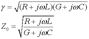
where γ is the complex propagation coefficient, and Z₀ is the complex characteristic impedance.

R,L,G, and C may be frequency dependent. In practical transmission lines at HF and above the following assumptions are often appropriately used:

• inductance per unit length as constant (due partially to skin effect and a fully effective outer conductor));
• capacitance per unit length as constant;
• resistance per unit length is subject to skin effect and is proportional to the square root of frequency; and
  
• conductance per unit length is due to dielectric loss and is proportional to frequency.

Because of Skin Effect, the effective resistance of a round conductor of homogenous material and more than about three Skin Depths in radius, is proportional to the square root of frequency. Conductor losses in that case are proportional to square root of frequency.

The reversal of electric field in a lossy dielectric expends a certain amount of energy, and when excited by an alternating voltage, the dielectric loss is usually proportional to the number of times that the field reverses in a given time period. Dielectric Loss in that case is proportional to frequency.

Skin Effect is well developed where the conductor radius more than about three skin depths.

Solving the equation for γ reveals that conductor loss is approximately proportional to R where R<<ωL, and dielectric loss is approximately proportional to G where G<<ωC. For most purposes, error is usually acceptable where R<ωL/3 and G<ωC/3.

Fig 2: Loss characteristics of example coaxial lines

Fig 2 shows the conductor and dielectric component losses for two popular coaxial cables of similar overall diameter. Both cables have a nominal Z₀ of 50Ω, RG213 uses a solid polyethylene dielectric and LMR400 uses a foamed polyethylene dielectric which has lower dielectric loss but more importantly a larger diameter centre conductor which reduces conductor loss.

As a result of the HF characteristics of the conductor and dielectric materials described above, Matched Line Loss at HF and above is very well approximated by the model MatchedLineLoss(dB)=k₁*f^0.5+k₂*f.

Taking RG213 as an example, MatchedLineLoss(dB)=5.929e-6*f^0.5+8.234e-11*f. The model is limited in this case to frequencies above:

• 30kHz for well developed Skin Effect; and
• 17kHz so that loss is proportional to R (R<ωL/3).

The lower frequency limit for application of the loss model depends on the line characteristics.

Materials exceptions

Note that not all materials are ideal in the sense discussed above, for example:

• conductors that are not homogenous, or very small diameter conductors might not have well developed skin effect, and may not exhibit R∝f^0.5;
• dielectric materials may exhibit a different loss factor at different frequencies; and
  
• energy coupled through ineffecitive shield structures.

The model is very suited to common practical coaxial cables with copper conductors and solid or foamed Polythene dielectric used at HF and above. The vast majority of commonly used RF grade coaxial cables fall into this category. Note though that some types of cables may have shield structures that are not fully effective at higher or lower frequencies (open weave braid, and thin metalised plastic shields respectively).

The model may not predict behaviour of cables with copper clad steel, tinned, or silver plated steel centre conductors well at HF because the Skin Effect criteria are violated (cladding or plating thickness not greater than three skin depths). Cables with small diameter conductors, even though homogenous, may not satisfy the skin depth requirement at lower frequencies.

Developing a loss model from measured Matched Line Loss

Line specifications usually include Matched Line Loss measured at a range of frequencies. Measured transmission line loss for a line terminated in its nominal Z₀ is usually a good fit to the model MatchedLineLoss(dB)=k₁*f^0.5+k₂*f. Measured loss vs f can be used to find k₁,k₂ values for the loss model (MatchedLineLoss(dB)=k₁*f^0.5+k₂*f) such that the residual sum of squares of error (SSE) is minimised.

In the case of a simple transmission loss test, strictly speaking, the line is not usually perfectly matched for, amongst other reasons, Z₀ is a function of frequency for most practical lines and is not usually exactly equal to |Z₀|+j0. This overestimates loss, though the error introduced is usually relatively small and its contribution is usually insignificant compared to other error sources (eg manufacturing tolerances, temperature variation etc), and the model remains a good predictor of line behaviour for most practical lines at HF and above.

It is important to identify measurements at lower frequencies that significantly depart from the loss model. These will have significant difference from the value predicted by the model, and exclusion of them from the model will reduce the residual SSE.

Note that many manufactures publish data obtained from the loss model rather than the raw measurement data, extremely low residual SSE is a good indicator.

Developing a RLGC model

The valid loss model along with nominal Z₀ (R_n)  and velocity factor vf (both obtainable from manufacturer's data, or by measurement) can be used to determine R(f), L, G(f) and C.

Solving the RLGC model

RF Transmission Line Loss Calculator uses a table of k₁,k₂ obtained from published or measured data at HF and above, and is a flexible tool for solution of the transmission line equations.

In some cases, data points at lower frequencies are excluded because they are a bad fit to the loss model. This has only occurred with coaxial cables that use copper clad steel (CCS) or plated steel inner conductors. The effect is not limited to coaxial cables, the effect should also be exhibited by two wire lines using CCS conductors at lower frequencies.

The calculated loss model reveals the underlying model for R∝(f^0.5); and G∝(f). These R and G values are used, along with nominal Z₀ and velocity factor to solve the Telegrapher's Equation to calculate Z₀, γ and then Matched Line Loss, and loss under mismatched conditions, etc.

RF Two Wire Transmission Line Loss Calculator calculates R and G from user input data, and then uses the same algorithms as explained above for RF Transmission Line Loss Calculator.

Examples

Example 1

(Parmley 2009) grappled with trying to estimate Zo of some 'zip cord' from various measurements. He reported measured velocity factor, conductor diameter, estimated Zo, and calculated loss based on some impedance measurements of stubs.

Fig 3:

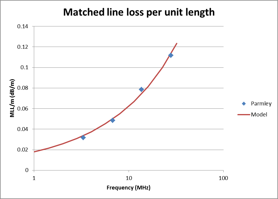Parmley tabulates calculated matched line loss, shown per metre in Fig 3 above. A regression matched line loss model was derived from the four data points and is shown, the loss model is MLL/m=1.7e-5f^0.5+8.4e-10f (MLL in dB, f in MHz).

The derived constants allow constructing a model in TWLLC as shown above. Conductor conductivity is low at about 20% of a round copper conductor of the same size (perhaps the wire was tinned), and the Loss Tangent of the dielectric is 0.0065 (which seems a little low).

It can be seen from the output of TWLLC above that Zo is about 150Ω, and loss in a half wavelength with 70+j0Ω load at 14MHz is 0.73dB.

Construction of the TWLLC model highlights that the Parmley's performance figures are better than can be explained by plain copper conductors and typical PVC insulation. The thrust of Parmley's article is that Zip cord may not be as bad as made out by some commentators, however it appears his reports of line loss may be a little optimistic.

Example 2

(Hall 1979) also grappled with characterising a non-traditional cable, a Zip cord type 14-118-2G42. Hall made measurements and reported #18 conductors, PVC insulation, Zo=105Ω at 15MHz, vf=0.7, and matched line loss at 15MHz of 4.1dB/100'.

Fig 5:

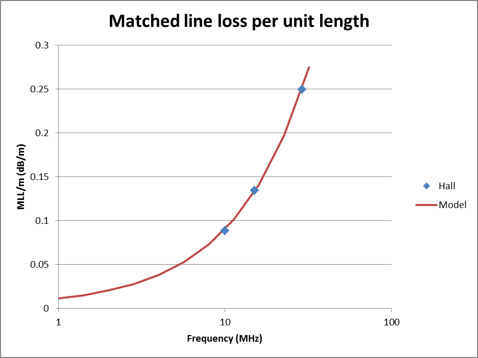Hall gives measured attenuation at three frequencies, shown per metre in Fig 5 above. A regression matched line loss model was derived from the four data points and is shown, the loss model is MLL/m=3.1e-6f^0.5+8.0e-9f (MLL in dB, f in MHz).

The derived constants allow constructing a model in TWLLC as shown above. Conductor conductivity is six times that of copper of the same size which is unrealistic, and the Loss Tangent of the dielectric is 0.063 (almost ten times that of Example 1, and perhaps high).

The model gives a line loss of 1.0dB under the mismatch conditions of a nominal 70+j0Ω load and half wavelength of line at 14MHz.

By contrast with Parmley's model, this model indicates conductor conductivity better than copper, a more realistic Loss Tangent, and higher loss despite using larger conductors (though Zo is lower).

Making measurements of open wire line is quite challenging. Hall noted in his article that results were affected by proximity of people to the line, which raises questions about the extent of radiation and its effect on results, and the implied conductor conductivity is unrealistically low.

Example 3

(Smith 2001) made a series of measurements of Zip cord and published his results on Usenet.

Fig 7:

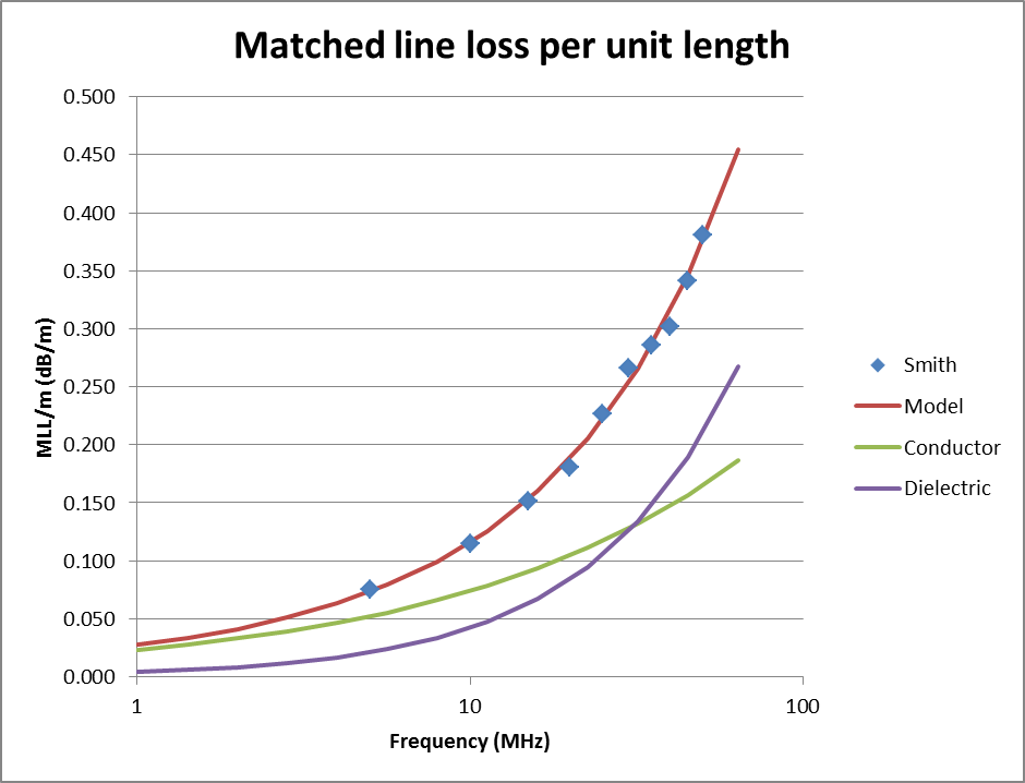Fig 7 above shows the measured matched line loss. A  regression matched line loss model was derived from the ten data points and is shown, the loss model is MLL/m=2.3e-5f^0.5+4.2e-9f (MLL in dB, f in MHz). The conductor and dielectric loss components of the model loss are also in Fig 7, and it can be seen that whilst dielectric loss is relatively low at 1MHz, it overtakes conductor loss at about 30MHz. Measurements made well above or well below this cutover might not capture well the effects of both kinds of loss.

The derived constants allow constructing a model in TWLLC as shown above. Conductor conductivity is about 7% that of copper of the same size, and the Loss Tangent of the dielectric is 0.03 (almost five times that of Example 1).

The model gives a line loss of 1.1dB under the mismatch conditions of a nominal 70+j0Ω load and half wavelength of line at 14MHz.

By contrast with Parmley's model, this model indicates conductor conductivity poorer than copper, a more realistic Loss Tangent, and higher loss despite using larger conductors (though Zo is lower). 

Example 4

(Hunt nd) reported measurements of three fabricated two wire lines.

Table 1 above shows the three cases, including Hunt's measured vf and Zo. The relative permittivity of the composite dielectric can be calculated from vf as ε_r=vf^-2. Using the stated dimensions and ε_r calculated from Hunt's measured vf, Zo was calculated using TWLLC and is reported in the table.

The calculated figures for the second and third case reconcile with Hunt's measured Zo.

 The first case uses a pair of conductors tied together with plastic zip ties every 100mm, it is unlikely that the conductors are touching through their entire length, the measured Zo and vf combination is attributable to a much wider spacing (predicted also by Hunt's own calculation tool), so it is unlikely that the line is uniform.

Note that TWLLC's estimate of line loss for cases two and three would not be good, as the RF resistance of the braided conductor will be considerably higher than for the plain conductor assumed by TWLLC.

None of these represent a good way to achieve a low loss low Zo line for the Hexbeam application. A pair of air spaced square section aluminium tubes is a practical solution though, eg 20mm tubes with 4mm spacing delivers Zo about 50 ohms, though it would need to be housed in a weatherproof housing to prevent rain changing its characteristics significantly (as for most open wire lines).

Example 5

John Oppenheimer (KN5L) made a series of measurements with a Rigexpert AA-54 of a twisted pair transmission line fabricated from a pair of 0.65mm (#22) stranded silver plated copper conductors with PTFE insulation. Estimated Ro was 112Ω.

The measurements include input R as series resonances of 30.48m (100') of line with o/c and s/c termination. The R value can be used with Zo to estimate matched line loss. In total, there were 10 datapoints.

Fig 9:

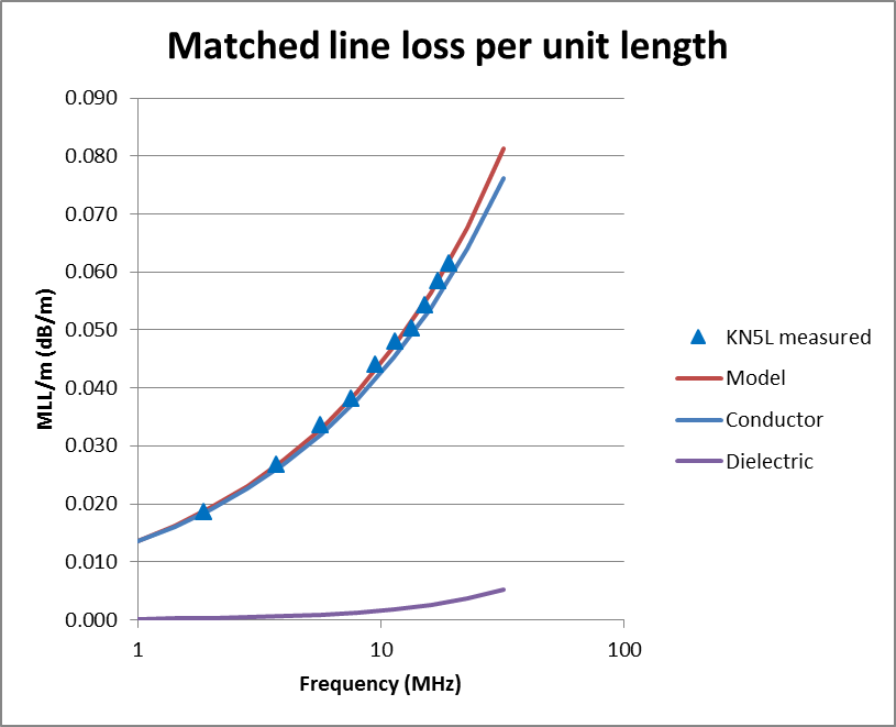Fig 9 above shows the measured matched line loss. A  regression matched line loss model was derived from the ten data points and is shown, the loss model is MLL/m=1.34622E-05f^0.5+1.60374E-10*f (MLL in dB, f in MHz). The F statistic for the regression model is 130,000, and extremely good statistical outcome.

Model dielectric and conductor losses are broken out and plotted. Comparison with Fig7 shows how poor flexible PVC insulated cable is at RF compared to PTFE. At 10MHz, this line has less than half the MLL of ZIP cord despite the ZIP cord having conductors of about twice the diameter.

This example demonstrates that an adequate set of measurements from a mid range antenna analyser can produce very good results.

Once Ro, vf and the loss model are know, ATLLC can be used for solutions.

Fig 10 shows the output of ATLLC for a tuned feeder for a 14MHz centre fed dipole which has been shortened to create a standing wave that can deliver the desired input impedance of 50+j0Ω.

Conclusions

The loss model MatchedLineLoss(dB)=(k₁*f^0.5+k₂*f)*l is a good model for practical transmission lines using homogenous conductors and quality materials at HF and above.

Fitting characterisation measurements to the loss model can be a worthwhile measure in validating those measurements, and providing a more generic model for predictive purposes.

Links / References

• Clarke, R N. 2005. Tables of Physical & Chemical Constants (16th edition 1995). 2.1.4 Hygrometry. Kaye & Laby Online. Version 1.0 (2005) www.kayelaby.npl.co.uk (accessed 18/11/12).
• Hall, J. Mar 1979. Zip-cord antennas - do they work? In QST Mar 1979 p31.
• Hunt, S. nd. Twin feed experiment. http://www.karinya.net/g3txq/twin_feed/ (accessed 24/06/12).
• Parmley, W. Mar 2009. Zip cord antennas and feedlines for portable applications In QST Mar 2009 p36.
• Smith, J. Oct 2001. Postings to group rec.radio.amateur.antennas. Usenet 2001.
• Figure-8 flex used as RF transmission line
• PVC insulated feed line on HF
• TWLLC
• TLLC

Changes

© Copyright: Owen Duffy 1995, 2021. All rights reserved. Disclaimer.