Sydney harbour is a beautiful place

One of the trips I am known to take is to Manly for lunch.

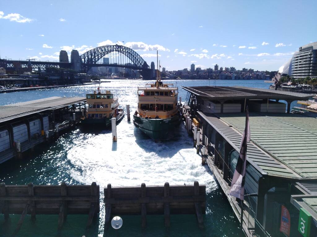
Above is a pic taken whilst waiting for the train home at Circular Quay. On the right is the ferry Freshwater arriving from Manly. The Opera House is just visible on the right north of the ‘toaster’ (one of the eyesores on the harbour).

It was a sparkling day on the harbour (Port Jackson) which bought back memories of many happy days boating and sailing, it is a beautiful waterway.

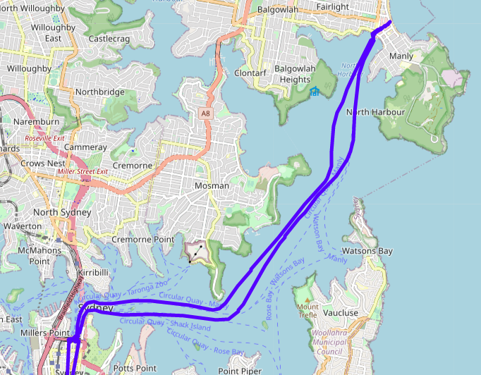
Manly is about 30min north east, 12km over the water, just on the north side of Sydney heads.

It is challenging to get pics on the ferry as tourists push their phone in front of your face to take videos, 5 to 10 minutes as a time.

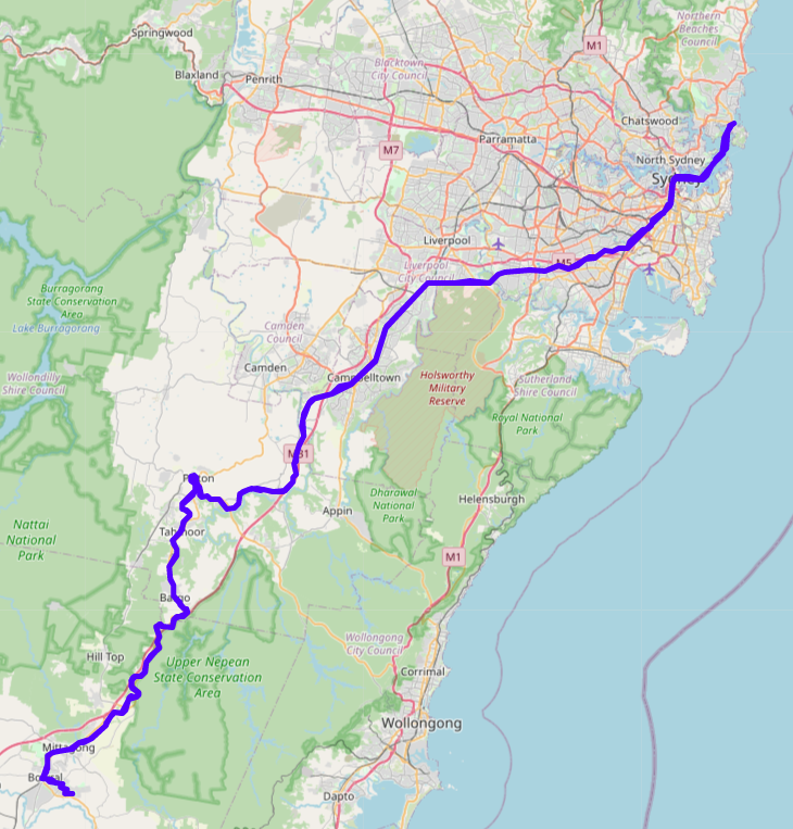
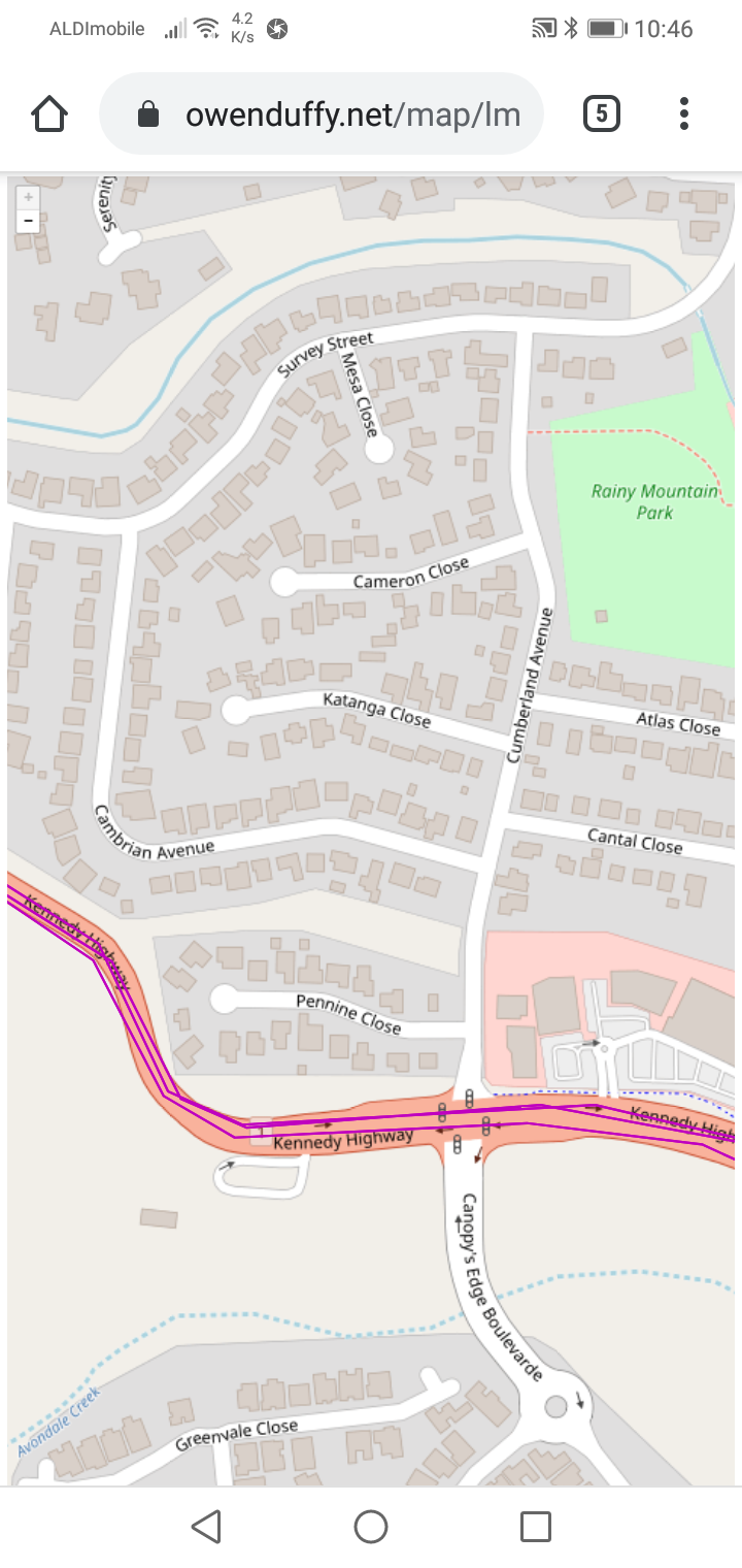
Above, the route is from home to Bowral station by car, diesel train (Endeavor railcar) to Central, electric train on the Sydney underground to Circular Quay, and ferry to Manly. The return journey was similar but electric train from Circular Quay to Campbelltown then diesel train to Bowral. The round trip is just on 300km and nearly three hours for each direction of travel.

An interactive zoomable map is available. Zooming in around Sydney and a little south will show track jumps due to underground rail.

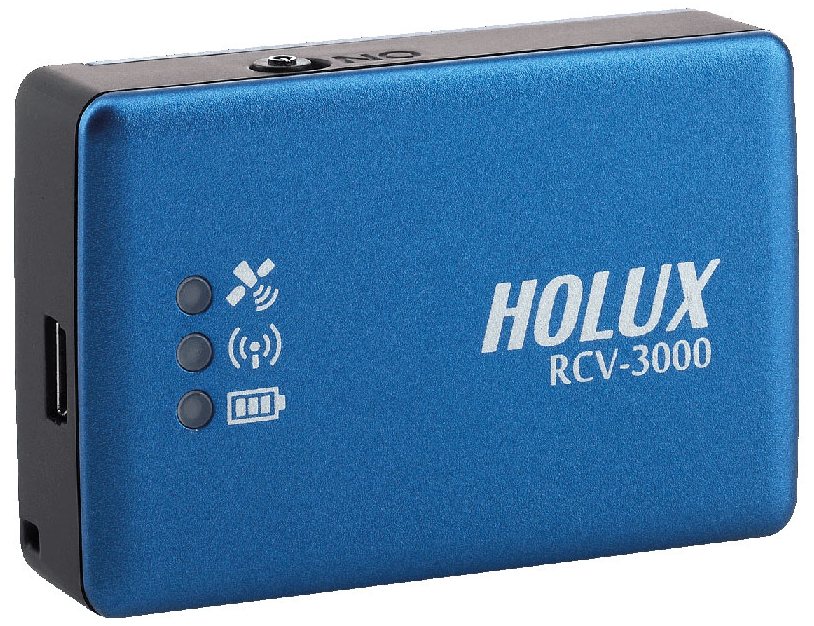
The track was captured with a Holux RCV-3000 GPS logger, logs downloaded with BT747 (Chinese firm Holux is defunct and so is their application which is now locked out of its maps provider).

Leaflet / OpenStreetMap map rendering on devices with tiny pixels

I wrote an application that presents maps on a webpage using Leaflet and OpenStreetMaps, and some readers commented that the text was hard to read on their devices.

It turns out that this issue seems present on devices with high resolution small screen (ie high pixels/mm or small pixel size).

The reports raise the question of whether it is the compatibility of the device and the user’s Visual Accuity (VA).

VA is often assessed on the familiar Snellen chart which has characters of a 5×5 grid and normal vision is indicated by reading characters that subtend 5 minutes of arc (MOA), or 1MOA for each ‘pixel’ (px).

An example phone screen calculation

My Huawei dub-lx2 has a screen height of 1520 px and 144mm, so the px size is 95µm. Keep in mind that the size of this pic may be much smaller on the phone that on your viewing device. Continue reading Leaflet / OpenStreetMap map rendering on devices with tiny pixels

Simsmith bimetal line type – revision #1

This article is a revision of an article Simsmith bimetal line type for Simsmith v17.2 and revisions to my own model for current distribution in a conductor.

This article discusses various measurements and models of Wireman 551 windowed ladder line, including adapting Simsmith’s bimetal line type to bear on the problem.

Measurements

A starting point for characterising the matched line loss (MLL) of the very popular Wireman 551 (W551) windowed ladder line is the extrapolation of measurements by (Stewart 1999) to 1.8MHz. Since the measurements were made at and above 50MHz where the W551 has copper like performance, this is likely to underestimate actual MLL and such wide extrapolation introduces its own uncertainty. Nevertheless, the datapoint is MLL=0.00227dB/m.

This is a revision of an article written in Feb 2020, capturing revision of Simsmith to v17.2 and revision of my own current distribution model.

Dan Maquire recently posted a chart summarising measurements of these lines.

For the purposes of this article, let’s tabulate the MLL at 1.8MHz in dB/m. Continue reading Simsmith bimetal line type – revision #1

A model of current distribution in copper clad steel conductors at RF – capturing conductor curvature

A model of current distribution in copper clad steel conductors at RF laid out a model for current distribution, though ignoring curvature of the conductor in calculating current density vs depth.

A model for current distribution in a conductor is that for a homogenous conducting half space with surface current parallel to the interface. Current density at depth d is given by the expression \(J_r=J_R\frac{J_0(kr)}{J_0(kR)}\) where δ is the skin depth \(δ=(ω \cdot µ \cdot σ)^{0.5}\) and \(k=\frac{1-\jmath}{\delta}\), σ is the conductivity). This takes into account curvature of the conductor surface, albeit with slower compute time.

Let’s compare the two algorithms on a test case at 1.8MHz being copper cladding of 67µm copper over a steel core for an overall diameter of 1.024mm (#18).

Above is a stacked image, the simpler algorithm is the feint plot.

There is a quite small difference in this case. When the expected loss of 400Ω line using the conductor is calculated, the result with the simpler algorithm is 1.3% less than the later one using the Bessel distribution.

Distance to fault in submarine telegraph cables ca 1871 – the leap expanded

Distance to fault in submarine telegraph cables ca 1871 gave a mathematical explanation of the location of fault…

Now it is in terms of the three known values u,v,w and unknown x.

\(w(v-2x+u)=(v-2x+u)x+(v-x)(u-x)\\\)

\(x^2-2wx+vw+uw-uv=0\) from which you can find the roots.

\(x=w – \sqrt{(w-v)(w-u)}\\\)

I have been asked to expand the last ‘leap’.

So we have \(x^2-2wx+vw+uw-uv=0\) which is a quadratic, a polynomial of order 2.

The solution or roots of a quadratic \(ax^2+bx+c=0\) are given by \(x=\frac{-b \pm \sqrt{b^2-4ac}}{2a}\).

So, for our quadratic \(a=1, b=-2w,c=vw+uw-uv\), so \(x=\frac{2w \pm \sqrt{(2w)^2-4(vw+uw-uv)}}{2}\).

Dividing the top and bottom by 2 we get \(x=w \pm \sqrt{w^2-(vw+uw-uv)}\) which can be rewritten as \(x=w \pm \sqrt{(w-v)(w-u)}\).

We want the lesser square root \(x_-=w-\sqrt{(w-v)(w-u)}\) because x must be less than w, a constraint of the physical problem.

So when measurements gave \(v=1040 \Omega\) and \(w=970 \Omega\) we can calculate that the distance to fault is the lesser root, 210.3km from Newbiggen-by-the-sea. (The greater root would imply a -ve value for x or y which is not physically possible.)

Review of MXITA SMA-8

The MXITA SMA-8 is a low cost torque wrench for 8mm, specifically for SMA connectors. It has an adjustable calibration, supplied at 1Nm but easily adjusted down to 0.6Nm to suit common brass SMA connectors, especially of doubtful quality.

I bought this after seeing several recommendations on a nanoVNA forum.

Above is the factory pic of the SMA-8. Continue reading Review of MXITA SMA-8

The ZS6BKW five band antenna – discussion of an NEC model

Origins

(Austin 1987) described a multiband HF antenna that is very popular with hams some thirty years later.

In his article, Austin explained the characteristic of a single wire multiband antenna with a series section matching transformer. The geometry is quite similar to the G5RV with hybrid open wire and coax feed, but Austin pursued lengths of the dipole legs, and matching section length and Zo to optimise VSWR50.

The design was never an ‘all band’ antenna, but rather a multiband antenna with low feed point VSWR50 on several bands. Austin tabulated the frequency relationship of the optimised bands for the case of a 400Ω matching section, and they were in the ratio of 1:1.97:2.52:3.47:4.04. If the first frequency was chosen to be 7.2MHz, the other centre frequencies would be 14.2, 18.1, 25.0 and 29.1MHz.

NEC model

To give insight into behaviour of the ZS6BKW I have built and NEC-4.2 model of a ZS6BKW with dipole 28.5m (L1) of 2mm dia copper wire at height of 10m above ‘average’ ground (σ=0.005 εr=13), and 13.44m (L2) electrical length of 400Ω lossless transmission line. L2 was tweaked to optimise alignment of the VSWR50 response with the ham bands. The model assumes no feedline common mode current.

Above is the VSWR50 response of the model from 3-30MHz. Minimum VSWR near the nominated five bands is quite low. Note that VSWR50 at 80m is quite poor. Continue reading The ZS6BKW five band antenna – discussion of an NEC model

Distance to fault in submarine telegraph cables ca 1871

In the early days of submarine telegraph cables, the cable technology was a single core steel wire wrapped in gutta-percha worked against ground. Now the gutta-percha was not a uniform or durable insulation and leaks to ground (sea) were inevitable, and when the leakage became sufficient the cable could not longer be used and had to be repaired.

The earliest method of locating a cable fault was a binary chop… which would mean deploying a cable ship, grapnelling for the cable, hauling it to the surface with a special dividing cut and hold grapnel that severed the cable when tension was too great, buoying off one end and steaming back to the other to haul it on board, clean it up and test to the far cable station. New cable was spliced and the cable ship steamed back to find the buoy and pull that end on board, clean and test to the other end. This was done to localise the fault, and eventually replace a fault section of cable. During this longish period, the cable was out of service. Continue reading Distance to fault in submarine telegraph cables ca 1871

nanoVNA – tuning stubs using TDR mode

From time to time I have discussions with correspondents who are having difficulties using an antenna analyser or a VNA to find / adjust tuned lengths of transmission lines. I will treat analyser as synonymous with VNA for this discussion.

The single most common factor in their cases is an attempt to use TDR mode of the VNA.

Does it matter?

Well, hams do fuss over the accuracy of quarter wave sections used in matching systems when they are not all that critical… but if you are measuring the tuned line lengths that connect the stages of a repeater duplexer, the lengths are quite critical if you want to achieve the best notch depths.

That said, only the naive think that a nanoVNA is suited to the repeater duplexer application where you would typically want to measure notches well over 90dB.

Is it really a TDR?

The VNA is not a ‘true’ TDR, but an FDR (Frequency Domain Reflectometer) where a range of frequencies are swept and an equivalent time domain response is constructed using an Inverse Fast Fourier Transform (IFFT).

In the case of a FDR, the maximum cable distance and the resolution are influenced by the frequency range swept and the number of points in the sweep.

\(d_{max}=\frac{c_0 vf (points-1)}{2(F_2-F_1)}\\resolution=\frac{c_0 vf}{2(F_2-F_1)}\\\) where c0 is the speed of light, 299792458m/s.

Let’s consider the hand held nanoVNA which has its best performance below 300MHz and sweeps 101 points. If we sweep from 1 to 299MHz (to avoid the inherent glitch at 300MHz), we have a maximum distance of 33.2m and resolution of 0.332m. Continue reading nanoVNA – tuning stubs using TDR mode

NEC sez…

I note the common introduction to online posts being NEC says, according to NEC, and the like.

Readers should take this to mean that the author denies their contribution in making assumptions and building the model, and the influence on the stated results.

It is basically a disclaimer that disowns their work. Continue reading NEC sez…