Optimum receive system noise figure for given ambient noise – Flex 6700

This article is a follow up to Optimum receive system noise figure for given ambient noise – Flex 6600 using data published at (Farson 2014) to make similar estimates for the Flex 6700.

How to determine the amount of RF Preamp gain to apply for band conditions suggests that the 6700 figures might also apply to the 6500 and 6400(M).

Farson gives a table of MDS in 500Hz bandwidth figures for the 6700 on certain bandws, including MDS for 4 RF Gain configurations, 0, 10, 20, and 30dB.

Above is Farson’s data with my chosen RF Gain option (selected for SND<3dB) and calculated values in yellow and orange for: Continue reading Optimum receive system noise figure for given ambient noise – Flex 6700

Optimum receive system noise figure for given ambient noise – Flex 6600

Gerald Youngblood (K5SDR) of FlexRadio wrote of optimal receiver noise figure relationship to antenna noise in a blog posting about SDR receivers.

This article discusses that posting in the context of linear receivers, ie effects of intermodulation distortion are not included.

His gives the following advice:

For optimal weak signal performance near the atmospheric (antenna) noise floor you want your receiver noise floor (sensitivity/MDS) to be 8 to 10 dB below the noise coming from the antenna.  For strong signal reception, less sensitivity is almost always better.

The terminology is not industry standard, but that is quite  usual for hams who have a need to redefine well known terms, and this is really loose with implied equivalence (eg sensitivity/MDS).

ITU-R P.372-14 speaks of natural noise as including atmospheric noise due to lightning, and also speaks of man made noise.

It is likely Youngblood is actually talking about man made noise since he uses man made noise figures from an earlier revision of P.372.

Optimal is a compromise between weak signal performance (ie S/N degradation due to internal receiver noise) and handling of strong signals that might clip in the ADC of an SDR receiver.

He gives a table of measured MDS (minimum discernable signal, which actually is synonymous with Noisefloor) for recommended configurations of a Flex 6600 radio on several bands.

Above is Youngblood’s data with my calculated values in yellow and orange for: Continue reading Optimum receive system noise figure for given ambient noise – Flex 6600

Minimum ambient noise level – ITU-R P.372-13 guidance

Comments were received from some readers of the article S/N degradation is related to external noise level and receive system internal noise.

Essentially, two questions were asked:

  • what is the minimum HF ambient noise level; and
  • explain observation of lower HF ambient noise level.

What is the minimum ambient noise level?

Above is Fig 2 from ITU-R P.372-13 which shows some key components of total ambient noise. The solid line is entitled “minimum noise level expected”, and it is a combination of curves B, C and D. Above 0.7MHz, only curves C and D are at play. Continue reading Minimum ambient noise level – ITU-R P.372-13 guidance

S/N degradation is related to external noise level and receive system internal noise

A question that arises from time to time is what is the minimum receiver noise figure for a given application.

This discussion considers the question applied to linear receivers, ie receivers with zero intermodulation distortion (IMD) and other non ideal characteristics, other than their internal noise which can be described by their Noise Figure (NF).

By definition, NF is the amount by which the component or system degrades the SNR, so in dB it is the difference in the S/N in to S/N out. Implicit in that definition is that it is based on source internal noise of 290K equivalent.

HF example

So for example lets say a receiver with equivalent noise bandwidth 2000Hz measures sensitivity of -125dBm for 10dB S/N out. We can calculate the noise in 2000Hz bandwidth from a 290K source to be -141dBm, and therefore the input S/N is -125 – -141 = 16dB. The ratio of the input S/N to output S/N is the difference in those in dB, 16-10=6dB. The NF is 6dB. We can also calculate an equivalent internal noise temperature of (10^(6/10)-1)*290=865K.

By convention, ambient noise (or external noise) is expressed in Kelvins, or dB wrt 290K. That does not imply that an antenna contributes exactly 290K. Continue reading S/N degradation is related to external noise level and receive system internal noise

Equivalent noise bandwidth – IC-7300 CW Rx Filter2 – (500Hz sharp)

For a lot of experiments, knowledge of the Equivalent Noise Bandwidth (ENB) of a receiver is necessary. The ENB is the bandwidth of an ideal rectangular filter with the same gain as some reference frequency.

Though filters are often specified in terms of bandwidth at x dB down, that metric is of relatively little value, the x is often 6dB but not always, the filters depart significantly from ideal or even common response.

In brief, a white noise source is connected to the receiver input, Filter2 (nominal 500Hz bandwidth sharp response) selected and set to standard PBT, and the audio output captured on a PC based audio spectrum analyser, Spectrogram 16 in this case.

Spectrogram is set to integrate over 30s to average the variations due to the noise excitation. The resulting graph and text spectrum log are saved.

The method is explained in detail at Measure IF Bandwidth.

Above is the spectrum plots, as receivers go this is relatively flat.
Continue reading Equivalent noise bandwidth – IC-7300 CW Rx Filter2 – (500Hz sharp)

Equivalent noise bandwidth – IC-7300 SSB Rx Filter2 – (2400Hz sharp)

For a lot of experiments, knowledge of the Equivalent Noise Bandwidth (ENB) of a receiver is necessary. The ENB is the bandwidth of an ideal rectangular filter with the same gain as some reference frequency, 1kHz is usually specified for SSB telephony receiver sensitivity measurement.

Though filters are often specified in terms of bandwidth at x dB down, that metric is of relatively little value, the x is often 6dB but not always, the filters depart significantly from ideal or even common response.

In brief, a white noise source is connected to the receiver input, Filter2 (nominal 2400Hz bandwidth sharp response) selected and set to standard PBT, and the audio output captured on a PC based audio spectrum analyser, Spectrogram 16 in this case.

Spectrogram is set to integrate over 30s to average the variations due to the noise excitation. The resulting graph and text spectrum log are saved.

The method is explained in detail at Measure IF Bandwidth.

Above is the spectrum plots, as receivers go this is relatively flat, lacking the usual tapering off above 1kHz (a technique to cheat on sensitivity specs).
Continue reading Equivalent noise bandwidth – IC-7300 SSB Rx Filter2 – (2400Hz sharp)

Anytone AT-D868UV: initial impressions

This article reports initial impressions of an Anytone AT-D868UV hand held VHF/UHF dual mode (DMR/FM) radio.

Above, the AT-D868UV, purchased for about A$225 incl post from Hong Kong. This model had a GPS though that is unusable on ham DMR networks, so it is wasted money if you like. They may be more expensive through online shops that collect GST, and of course in countries where tariffs are applied to make them great again, prices may be higher.
Continue reading Anytone AT-D868UV: initial impressions

Riding the RF Gain control – part 5

Every so often one sees advice from experts on how to operate a communications receiver or transceiver for SSB reception on the HF bands.

Very often that advice is to adjust AF Gain to max, and adjust RF Gain for a comfortable listening level. This is argued today to deliver the best S/N ratio, partly due to delivering the lowest distortion due to IMD in the receiver front end.

This is the last of a series of articles exploring and discussing the wisdom of that traditional advice. The preceding parts have examined a range of receiver types identifying their susceptibility to overload in one form or another, means of minimising the risk of overload, and effects of S/N ratio.

Most recommendations to intervene lack quantitative evidence to support the claimed benefits.

Let us quantitatively explore the advice on a modern receiver.

A quantitative example

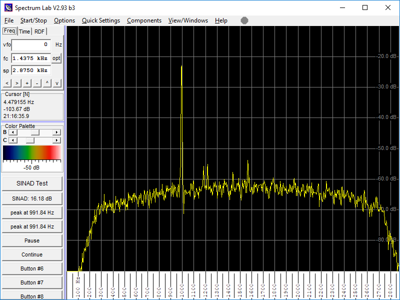
In this test, a modern budget priced receiver, an IC-7300, is used to evaluate SINAD (similar to S/N) on a steady signal off-air, trying initially the ‘sensible’ basic automatic setting to suit the 40m band, and then various preamp, attenuator and RFGAIN settings to try to win an improvement in SINAD.

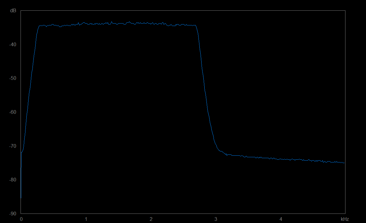
Above is a screenshot from SpectrumLab of a SINAD measurement on the IC-7300 setup normally for 7MHz (PREAMP OFF, ATTENUATOR OFF, RFGAIN MAX). Without signal, the S meter indicates around S4, with signal the S meter readings is around S7 and SINAD is around 16dB (it dances around a few tenths of a dB due to the combination of FFT bin size and integration interval). Continue reading Riding the RF Gain control – part 5

Riding the RF Gain control – part 4

This article continues on from Riding the RF Gain control – part 3 and explores the operating advice when applied to the next generation of receivers.

Direct sampling SDR

Lets jump a generation to the direct sampling SDR configuration.

In this category, I am covering receivers that do not convert the receive signal to an intermediate frequency, the ADC samples the signal at its off-air frequency.

The receivers may or may not have the following elements ahead of the ADC:

  • preamplifiers;
  • bandpass filters;
  • attenuators.

Because there may be no amplification prior to the ADC in some operating configurations, a voltage controlled attenuator may be used to prevent overflow of the ADC, this is the ‘analogue’ part of the AGC system. Continue reading Riding the RF Gain control – part 4

Riding the RF Gain control – part 3

This article continues on from Riding the RF Gain control – part 2 and explores the operating advice when applied to the next generation of receivers.

Conventional superheterodyne communications receiver with DSP demodulation.

The next generation of receivers was a conventional superheterodyne with a DSP based demodulation stage (initially at quite low Intermediate Frequency to suit the power of the available DSP chips).

Communications receivers were enhanced by replacement of the demodulators with a DSP performing demodulation digitally. The DSP sampled the IF signal and digitised it, and channel filtering and demodulation was performed ‘mathematically’ using the digital data stream as input.

There are two significant differences with this change:

  • receiver bandwidth can be determined by digitally synthesised passband filters in the DSP; and
  • first step in the DSP process is conversion of the IF signal to a digital stream in an analogue to digital converter (ADC).

Critically, the Analogue to Digital Converter (ADC) had an overflow point, and overflow of the ADC creates serious IMD and major degradation of received signal, overflow has to be prevented at all cost. To limit the power delivered to the ADC, a narrow ‘roofing’ filter usually preceded it, and the channel filter was digitally synthesised. Continue reading Riding the RF Gain control – part 3