Tag: Exploiting your antenna analyser

A correspondent wrote about the apparent conflict between Exploiting your antenna analyser #11 and Alan, K0BG’s discussion of The SWR vs. Resonance Myth. Essentially the correspondent was concerned that Alan’s VSWR curve was difficult to understand.

K0BG’s pitch

For convenience, here is the relevant explanation.

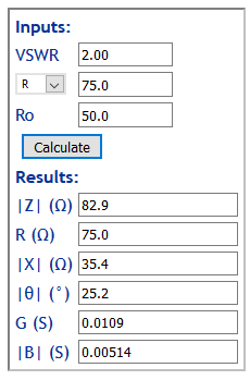
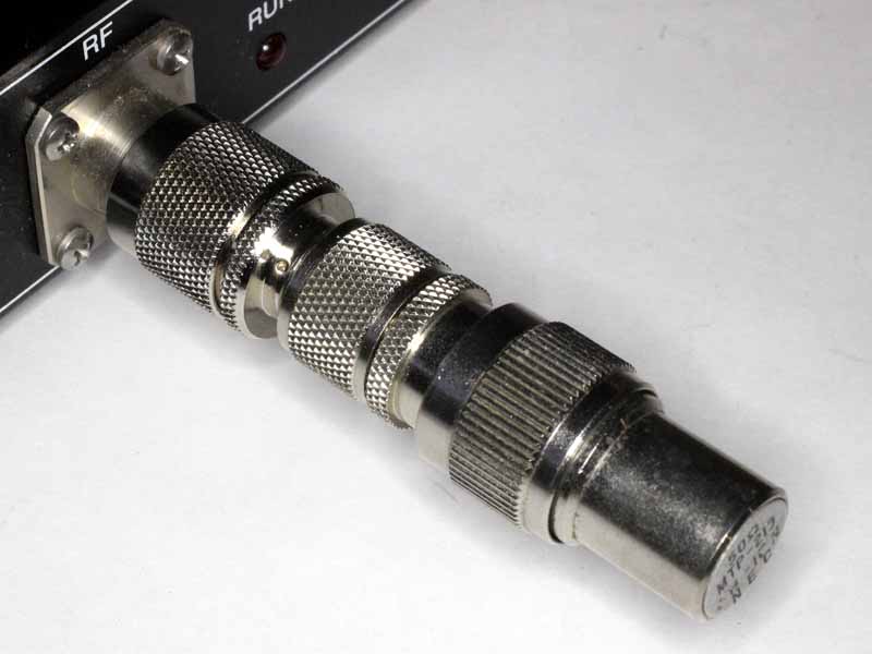
By definition, an antenna’s resonant point will be when the reactive component (j) is equal to zero (X=Ø, or +jØ). At that point in our example shown at left, the R value reads 23 ohms, and the SWR readout will be 2.1:1 (actually 2.17:1). If we raise the analyzer’s frequency slightly, the reactive component will increase (inductively) along with an increase in the resistive component, hence the VSWR will decrease, perhaps to 1.4:1. In this case, the MFJ-259B is connected to an unmatched, screwdriver antenna mounted on the left quarter panel, and measured through a 12 inch long piece of coax. This fact is shown graphically in the image at right (below).

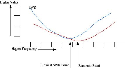
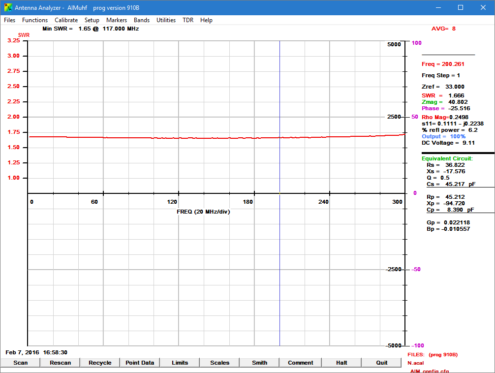
Note that the graph is unscaled, and that frustrates interpretation. The text is also not very clear, a further frustration. It is easy to draw a graph… but is the graph inspired by a proposition or is it supporting evidence. Continue reading Exploiting your antenna analyser #21

Finding resistance and reactance with some low end analysers #2

Exploiting your antenna analyser #8 was about finding resistance and reactance with some low end analysers that don’t directly display those values of interest. The article showed how to calculate the values starting with |Z| from the analyser and included links to a calculator to perform the calcs.

This article describes an extension to that calculator Find |Z|,R,|X| from VSWR,|Z|,R,Ro to use R, VSWR, and Ro as the starting point. Note that the sign of X and the sign of the phase of Z cannot be determined from this starting point, there just isn’t enough information.

You will probably not find the equation for |X|(R,VSWR,Ro) in text books or handbooks, and the derivation is not shown here but if there is interest, I may publish a separate paper.

Lets say you knew VSWR=2, R=75Ω, Ro=50Ω, what is |X|?

Above, entering the values in the calculator we find that |X|=35.4Ω. Continue reading Exploiting your antenna analyser #20

Critically review your measurements

A recent post on an online forum provides a relevant example to discussion of this subject.

I have personally seen ratios similar to 3:1 or higher at the feed point become 1:1 at the rig over 100 or so feet of coax cable.

First point is that in good transmission line, it takes an infinite length to deliver the observations made above. Less might deliver almost VSWR=1 at the input end of the line.

Let us consider a practical scenario, 100′ of RG58A/U with a load of 150+j0Ω at 14MHz, the load end VSWR₅₀ is 3, the input impedance is 32.50-j22.86Ω and input VSWR₅₀ is 2.01. In this scenario, the line loss is 2.5dB which might be unacceptable for some applications. Continue reading Exploiting your antenna analyser #19

Measure velocity factor of open wire line

One of the measurement tasks that one often encounters is to measure the velocity factor of a transmission line.

Often this is an indirect task of tuning a tuned line section, my method is to often measure some line off the role, find the velocity factor (vf), and use that to cut line for the tuned section making appropriate allowance for connectors etc.

Measuring vf for an open wire line includes all that is done for measuring vf of coax, but requires measures to ensure that common mode current does not affect measurement significantly.

To minimise common mode current effects, I will use two measures:

• a high common mode impedance Guanella balun; and
• form the line section being measured into a loose helix supported on some fishing line to spoil any common mode resonance.

Above is the balun used, it is described at Low power Guanella 1:1 balun with low Insertion VSWR using a pair of Jaycar LF1260 suppression sleeves. Continue reading Exploiting your antenna analyser #18

Optimising a G5RV with hybrid feed

(Varney 1958) described his G5RV antenna in two forms, one with tuned feeders, and the more popular form with hybrid feed consisting of a so-called matching section of open wire line and then an arbitrary length of lower Z0 coax or twin to the transmitter.

(Duffy 2005) showed that the hybrid feed configuration is susceptible to high losses in the low Z0 line as it is often longish, is relatively high loss line and operates with standing waves. Varney did offer two options for the low Z0 line: any length 72Ω twin or coax. Continue reading Exploiting your antenna analyser #17

Measure inductor using SOL calibration

At Measuring balun common mode impedance I showed a method of backing out the effects of a text fixture using the “subtract cable” facility of Antscope software with the Rigexpert AA-600.

Some analysers (including the AA-600) support SOL calibration of the instrument itself, and some support SOL calibration using the client software (Antscope in this case). This article demonstrates use of Antscope with SOL calibration to measure a small RF inductor which has similar characteristic to good Guanella 1:1 HF baluns.

The text fixture used for this demonstration is constructed on a SMA(F) PCB connector using some machined pin connector strip, and SMA(M)-SMA(M) and N(M)-SMA(F) adapters to connect to the AA-600.

Above is a pic of the test inductor in the test fixture with adapters. The test inductor 6 turns of 0.5mm PVC insulated wire wound on a BN43-202 binocular balun core. Continue reading Exploiting your antenna analyser #16

Measure MLL using the half ReturnLoss method – a spot test with a hand held analyser

At Exploiting your antenna analyser #14 I gave an explanation of the method of approximating MLL of a line section by taking the average half Return Loss with o/c and s/c terminations.

This article demonstrates the technique using the Rigexpert AA-600 analyser in hand held mode.

The task is to assess whether a section of RG58A/U coax has MLL at 3.5MHz similar to specification or not.

The specification loss of 10.13m of RG58A/U has MLL=0.29dB.

Above, the first test with an o/c termination. Return Loss is 0.4dB. Continue reading Exploiting your antenna analyser #15

Insertion Loss, Mismatch Loss, Transmission Loss

A correspondent asks about the effect of RCA connectors at HF on his proposed noise bridge. The question is very similar to that considered at Exploiting your antenna analyser #13 for UHF series connectors.

I have made a simple measurement of a BNC 50Ω termination (to check calibration) then inserted a BNC-RCA and RCA-BNC adapter.

Measurements of input impedance only for such an electrical short transmission line will not give useful data for determining TransmissionLoss which is the result of conversion of RF energy to heat. The measurements do give ReturnLoss and given that InsertionLoss=MismatchLoss+TransmissionLoss, they set a lower bound for InsertionLoss.

To jump to the chase, it also has a Smith chart plot up to 200MHz that suggests it might be well modelled by a TL segment of 30-35Ω.

Above is a plot of VSWR when Zref is adjusted for the flattest response from DC, and it can be seen that with Zref=33, response is quite flat to 200MHz. Continue reading Exploiting your antenna analyser #14

Insertion Loss, Mismatch Loss, Transmission Loss

A correspondent having read Exploiting your antenna analyser #12 asks whether the measurement provides evidence of loss of the connectors, and referred me to (Arther nd) where he reports some measurements of UHF series adapters and conclusions.

Duffy

Let’s deal with interpretations of my own measurements first.

Measurements of input impedance only for such an electrical short transmission line will not give useful data for determining TransmissionLoss which is the result of conversion of RF energy to heat. The measurements do give ReturnLoss and given that InsertionLoss=MismatchLoss+TransmissionLoss, they set a lower bound for InsertionLoss.

Above is a plot of ρ and ReturnLoss for the DUT. ReturnLoss curiously is plotted ‘upside down’ as ReturnLoss increases downwards… a quirk of AIM software, but remember that ReturnLoss in dB is +ve.
Continue reading Exploiting your antenna analyser #13

Is there a place for UHF series connectors in critical measurement at UHF?

Seeing some recent discussion by a chap who was trying to construct a low power 50Ω termination on a UHF series plug, it bought to mind the futility of using some kinds of connector for critical measurement above perhaps 100MHz.

There is a lot of conjecture about the nature of UHF series connectors, whether they act line a simple transmission line section with fairly uniform Zo, whether they are really just a lumped shunt capacitance, whether it is even important at UHF etc.

To illustrate the issue, I have assembled a simple test jig comprising an N(M)-UHF(F) adapter, UHF(M)-N(F) adapter and a 50Ω N termination (which was also used to calibrate the analyser. This set was assembled and plugged onto a calibrated AIMuhf analyser and swept from 1-500MHz… just into the UHF range (which is 300-3000MHz).

Above, the test jig.

Above is an expanded scale centre of the Smith chart of the sweep. Continue reading Exploiting your antenna analyser #12