Phase of s11 and Z

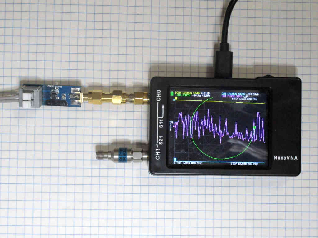
Antenna system resonance and the nanoVNA contained the following:

Relationship between angle of reflection coefficient and angle of impedance

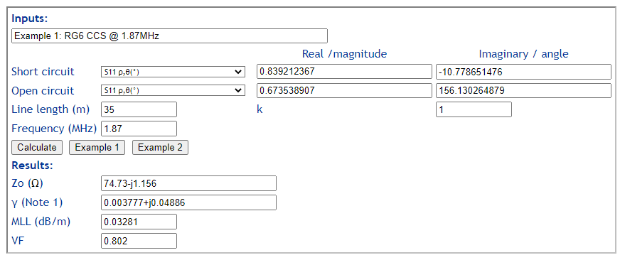
It was stated above that the angle (or phase) of s11 or Γ is not the same as the angle (or phase) of Z.

Given Zo and Γ, we can find θ, the angle of Z.

\(
Z=Z_0\frac{1+\Gamma}{1-\Gamma}\)

Zo and Γ are complex values, so we will separate them into the modulus and angle.

\(
\left | Z \right | \angle \theta =\left | Z_0 \right | \angle \psi \frac{1+\left| \Gamma \right | \angle \phi}{1-\left| \Gamma \right | \angle \phi} \\
\theta =arg \left ( \left | Z_0 \right | \angle \psi \frac{1+\left| \Gamma \right | \angle \phi}{1-\left| \Gamma \right | \angle \phi} \right )\)

We can see that the θ, the angle of Z, is not simply equal to φ, the angle of Γ, but is a function of four variables: \(\left | Z_0 \right |, \psi , \left| \Gamma \right |, \& \: \phi\) .

It is true that if ψ=0 and φ=0 that θ=0, but that does not imply a wider simple equality. This particular combination is sometimes convenient, particularly when ψ=0 as if often the case with a VNA.

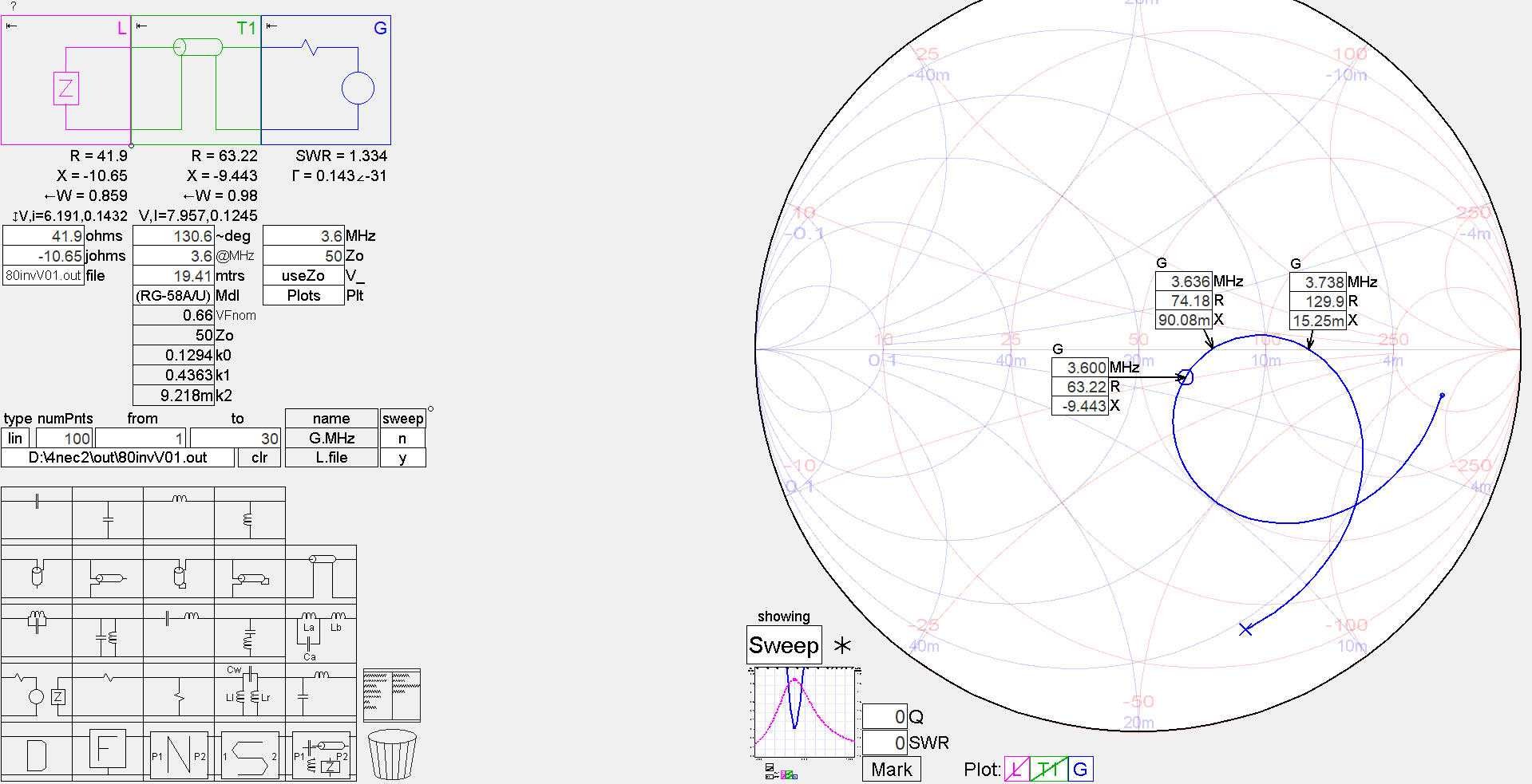
This article offers a simulation of a load similar to a 7MHz half wave dipole.

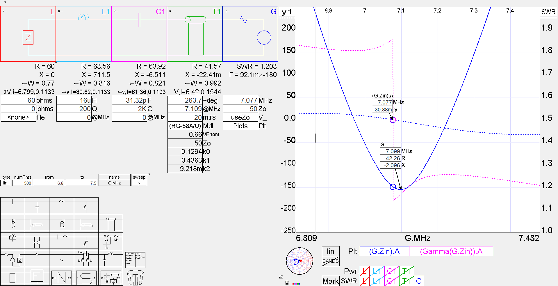
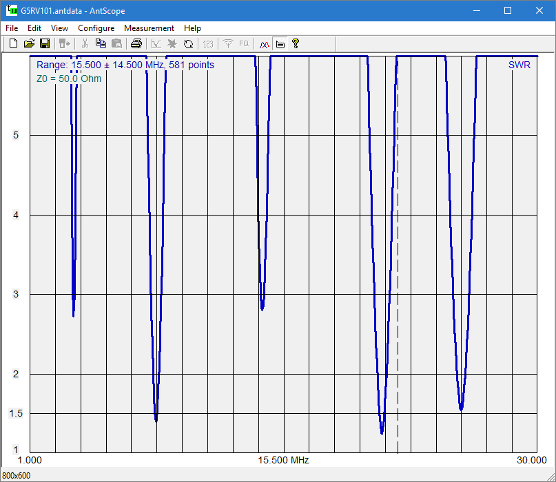
The load comprises L, L1, and C1 and the phase of s11 (or Γ) and phase of Z (seen at the source G) are plotted, along with VSWR. Continue reading Phase of s11 and Z

The quarter sized G5RV with hybrid feed

(Varney 1958) described his G5RV antenna in two forms, one with tuned feeders and the more popular form with hybrid feed consisting of a matching section of open wire line and then an arbitrary length of lower Zo coax or twin to the transmitter.

(Duffy 2005) showed that the hybrid feed is susceptible to high losses in the low Zo line as it is often longish, is relatively high loss line and operates with standing waves.

Lets look at measurement of a real antenna, broadly typical of the G5RV. The antenna measured is a G5RV rigged in Inverted V form, 11m height at the apex and around 8m at the ends. The feed line is 2mm diameter copper spaced 50mm with occasional plastic insulators.

To some extent, the measurements are dependent on the environment, and whilst there will be variation from one implementation to another, the measurements provide a basis for exposing the configuration challenge.

Screenshot - 01_05_16 , 19_33_56

Above is a plot of VSWR50 essentially at the lower end of the matching section and low Zo line. The measurement is made looking into 0.5m of RG142 and a Guanella current balun that uses about 1m of 110Ω pair, it is essentially the load end VSWR of a hybrid feed were it used. Continue reading The quarter sized G5RV with hybrid feed

Antenna system resonance and the nanoVNA

With the popularity of the nanoVNA, the matter of optimisation of antenna systems comes up and the hoary chestnuts of ham radio are trotted out yet again.

Having skimmed a presentation published on the net, an interesting example is presented of an 80m half wave centre dipole with feed line and various plots from the nanoVNA used to illustrate the author’s take on things.

The author is obsessed with resonance and obsessed with phase, guiding the audience to phase as ‘the’ optimisation target. Phase of what you might ask… all the plots the author used to illustrate his point are phase of s11.

A model for discussion

I have constructed an NEC-4.2 model of a somewhat similar antenna to illustrate sound concepts. Since NEC-4.2 does not model lossy transmission lines (TL elements), we will import the feed point data into Simsmith to include transmission line loss in the model.

Above is the Simsmith model. Continue reading Antenna system resonance and the nanoVNA

Calculate Loss from s11 and s21 – convenient online calculator

I often need to calculate loss from marker values on a VNA screen, or extracted from a saved .s2p file.

Firstly, loss means PowerIn/PowerOut, and can be expressed in dB as 10log(PowerIn/PowerOut). For a passive network, loss is always greater than unity or +ve in dB.

\(loss=\frac{PowerIn}{PowerOut}\\\)

Some might also refer to this as Transmission Loss to avoid doubt, but it is the fundamental meaning of loss which might be further qualified.

So, lets find the two quantities in the right hand side using ‘powerwaves’ as used in S parameter measurement.

s11 and s21 are complex quantities, both relative to port 1 forward power, so we can use them to calculate relative PowerIn and relative PowerOut, and from that PowerIn/PowerOut.

PowerIn

PowerIn is port 1 forward power less the reflected power at port 1, \(PowerIn=P_{fwd} \cdot (1-|s11|^2)\).

PowerOut

PowerOut is port 2 forward power times less the reflected power at the load (which we take to be zero as under this test it is a good 50Ω termination), \(PowerOut=P_{fwd} \cdot |s21|^2 \).

Loss

So, we can calculate \(loss=\frac{PowerIn}{PowerOut}=\frac{\frac{PowerIn}{P_{fwd}}}{ \frac{PowerOut}{P_{fwd}}}=\frac{1-|s11|^2}{|s21|^2}\)

Noelec makes a small transformer, the Balun One Nine, pictured above and they offer a set of |s11| and |s12| curves in a back to back test. (Note: back to back tests are not a very reliable test.) Continue reading Calculate Loss from s11 and s21 – convenient online calculator

Measure transmission line Zo – nanoVNA – PVC speaker twin

There are many ways to get a good estimate of the characteristic impedance Zo of a transmission line.

One method is to measure the input impedances of a section of line with both a short circuit and open circuit termination. From Zsc and Zoc we can calculate the Zo, and the complex propagation constant \(\gamma=\alpha + \jmath \beta\), and from that, MLL.

Calculation of Zo is quite straightforward.

The solution for γ involves the log of a complex number \(r \angle \theta\) which is one of the many possible values \(ln(r) + j \left(\theta + 2 \pi k \right)\) for +ve integer k. Conveniently, the real part α is simply \(ln(r) \). The real part of γ is the attenuation in Np/m which can be scaled to dB/m, and the imaginary part is the phase velocity in c/m. The challenge is finding k.

Measurement with nanoVNA

So, let’s measure a sample of 14×0.14, 0.22mm^2, 0.5mm dia PVC insulated small speaker twin.

Above is the nanoVNA setup for measurement. Continue reading Measure transmission line Zo – nanoVNA – PVC speaker twin

Measure transmission line Zo – nanoVNA – CCS RG6

There are many ways to get a good estimate of the characteristic impedance Zo of a transmission line.

One method is to measure the input impedances of a section of line with both a short circuit and open circuit termination. From Zsc and Zoc we can calculate the Zo, and the complex propagation constant \(\gamma=\alpha + \jmath \beta\), and from that, MLL.

Calculation of Zo is quite straightforward.

The solution for γ involves the log of a complex number \(r \angle \theta\) which is one of the many possible values \(ln(r) + j \left(\theta + 2 \pi k \right)\) for +ve integer k. Conveniently, the real part α is simply \(ln(r) \). The real part of γ is the attenuation in Np/m which can be scaled to dB/m, and the imaginary part is the phase velocity in c/m. The challenge is finding k.

Let’s take an example from recent measurements of 35m of CCS RG6 coax, and extract the s11 values recorded in saved .s1p files @ 1.87MHz. The saved data in MA format, magnitude and angle (in degrees).

Calculate Zo and gamma is flexible and can accept the MA format data directly.

Above, the results. Zo is 74.73-j1.156Ω, and matched line loss MLL is 0.03281dB/m. This MLL is quite a deal higher than you might find in many line loss calculators, they often fail on CCS cables. Continue reading Measure transmission line Zo – nanoVNA – CCS RG6

Nichols: The Two Bird Experiment

With the following introduction, (Nichols nd) tries to demonstrate some important principles. He says…

This really tests your understanding of transmission line theory.

Above is Nichols’ test setup, simple enough.

With the transmitter keyed, the transmatch is adjusted to show zero reflected power on Bird Wattmeter #1. Transmitter is then adjusted to generate exactly 100 watts of forward power indicated on Bird Wattmeter #1. Bird directional Wattmeter #2 indicates about 36 watts of REFLECTED power. (Charts are readily available to show that a 4:1 mismatch gives about 36% reflected power).

Continue reading Nichols: The Two Bird Experiment

nanoVNA – measure Transmission Loss – example 5

This article is demonstration of measurement of Transmission Loss in a section of two wire transmission line embedded in a common mode choke. The scenario is based on an online article  MEASURING DM ATTENUATION of YOUR CMC USING THE NANOVNA AND NANOVNA SAVER.

The reference article publishes measured attenuation or loss being -1.45dB @ 28.4MHz. Of course, the -ve value hints that the author is lost in hamdom where all losses MUST be -ve dB..

The meaning of loss in a generic sense (ie without further qualification) is \(loss=\frac{Power_{in}}{Power_{out}}\) and can be expressed in dB as \(loss_{dB}=10 log_{10}(loss)\).

Some might interpret the result to imply that \((1-10^{\frac{-loss}{10}})*100=28 \%\) of input power is converted to heat in the choke.

The result given (and corrected) as 1.45dB was taken simply from the nanoVNA \(|s21|\) result, and so it is actually InsertionLoss, not simply Loss.

What is the difference? Continue reading nanoVNA – measure Transmission Loss – example 5

Disturbing the thing being measured – coax line

An issue that often arises in online discussions inability to reconcile the VSWR indicated by a transceiver (or possibly an inline VSWR meter) and an antenna analyser.

Is this Segal’s law at play?

There are several common contributors including:

  • faulty, dirty, or not properly mated connectors and cables;
  • VSWR meters that are not accurate at low power levels; and
  • influence of the common mode current path on VSWR.

Continue reading Disturbing the thing being measured – coax line